What is Present Day Theoretical Chemistry About?
Structure
theory
For information about researchers posted after Oct. 1, 2009, please go to this link; it covers electronic structure, molecular
dynamics, and statistical mechanics.
A. Electronic structure theory describes the motions of the electrons and produces energy surfaces
The shapes and geometries of molecules, their electronic,
vibrational, and rotational energy levels and wavefunctions, as well
as the interactions of these states with electromagnetic fields lie
within the realm of structure theory.
In the Born-Oppenheimer
model of molecular structure, it is assumed that the electrons move
so quickly that they can adjust their motions essentially
instantaneously with respect to any movements of the heavier and
slower moving atomic nuclei. This assumption motivates us to view the
electrons moving in electronic wave functions (orbitals within the
simplest and most commonly employed theories) that smoothly "ride"
the molecule's atomic framework. These electronic functions are found
by solving a Schrödinger equation whose Hamiltonian
He contains the kinetic energy Te of the
electrons, the Coulomb repulsions among all the molecule's electrons
Vee, the Coulomb attractions Ven among the
electrons and all of the molecule's nuclei treated with these nuclei
held clamped, and the Coulomb repulsions Vnn among all of
these nuclei. The electronic wave functions yk
and energies Ek that result from solving the electronic
Schrödinger equation
He yk = Ek yk
thus depend on the locations {Qi} at which the nuclei are sitting. That is, the Ek and yk are parametric functions of the coordinates of the nuclei.
These electronic energies' dependence on the positions of the
atomic centers cause them to be referred to as electronic energy
surfaces such as that depicted below for a diatomic molecule where
the energy depends only on one interatomic distance R.
For non-linear polyatomic molecules having N atoms, the energy
surfaces depend on 3N-6 internal coordinates and thus can be very
difficult to visualize. A slice through such a surface (i.e., a plot
of the energy as a function of two out of 3N-6 coordinates) is shown
below and various features of such a surface are detailed.
The Born-Oppenheimer theory of molecular structure is soundly based in that it can be derived from a starting point consisting of a Schrödinger equation describing the kinetic energies of all electrons and of all N nuclei plus the Coulomb potential energies of interaction among all electrons and nuclei. By expanding the wavefunction Y that is an eigenfunction of this full Schrödinger equation in the complete set of functions { yk } and then neglecting all terms that involve derivatives of any yk with respect to the nuclear positions {Qi }, one can separate variables such that:
1. The electronic wavefunctions and energies must obeyHe yk = Ek yk
2. The nuclear motion (i.e., vibration/rotation) wavefunctions must obey
(TN + Ek) ck,L = Ek,L ck,L ,
where TN is the kinetic energy operator for movement of
all nuclei.
That is, each and every electronic energy state, labeled k, has a set, labeled L, of vibration/rotation energy levels Ek,L and wavefunctions ck,L .
Because the Born-Oppenheimer model is obtained from the full Schrödinger equation by making approximations (e.g., neglecting certain terms that are called non-adiabatic coupling terms), it is not exact. Thus, in certain circumstances it becomes necessary to correct the predictions of the Born-Oppenheimer theory (i.e., by including the effects of the neglected non-adiabatic coupling terms using perturbation theory).
For example, when developing a theoretical model to interpret the rate at which electrons are ejected from rotationally/vibrationally hot NH- ions, we had to consider coupling between two states having the same total energy:
1. 2P NH- in its v=1 vibrational level and in a high rotational level (e.g., J >30) prepared by laser excitation of vibrationally "cold" NH- in v=0 having high J (due to natural Boltzmann populations); see the figure below, and
2. 3S NH neutral plus an ejected electron in which the NH is in its v=0 vibrational level (no higher level is energetically accessible) and in various rotational levels (labeled N).
Because NH has an electron affinity of 0.4 eV, the total energies
of the above two states can be equal only if the kinetic energy KE
carried away by the ejected electron obeys:
KE = Evib/rot (NH- (v=1, J)) - Evib/rot (NH (v=0, N)) - 0.4 eV.
In the absence of any non-adiabatic coupling terms, these two
isoenergetic states would not be coupled and no electron detachment
would occur. It is only by the anion converting some of its
vibration/rotation energy and angular momentum into electronic energy
that the electron that occupies a bound N2p orbital in
NH- can gain enough energy to be ejected.
Energies of NH- and of NH pertinent to the autodetachment of v=1, J levels of NH- formed by laser excitation of v=0 J'' NH- .
My own research efforts have, for many years, involved studying negative molecular ions (a field in which Professor Ken Jordan is a leading figure) taking into account such non Born-Oppenheimer couplings, especially in cases where vibration/rotation energy transferred to electronic motions causes electron detachment as in the NH- case detailed above.
 |
|
|
|
|
My good friend, Professor Yngve Öhrn, has been active in attempting to avoid making the Born-Oppeheimer approximation and, instead, treating the dynamical motions of the nuclei and electrons simultaneously. Professor David Yarkony has contributed much to the recent treatment of non-adiabatic (i.e., non Born-Oppenheimer) effects and to the inclusion of spin-orbit coupling in such studies.
|
|
|
|
|
|
|
The knowledge gained via structure theory is great. The electronic
energies Ek (Q) allow one to determine (see my book
Energetic Principles of Chemical
Reactions) the geometries and relative energies of various
isomers that a molecule can assume by finding those geometries
{Qi ) at which the energy surface Ek has minima
![]() Ek
/
Ek
/![]() Qi
= 0, with all directions having positive curvature (this is
monitored by considering the so-called Hessian matrix
Qi
= 0, with all directions having positive curvature (this is
monitored by considering the so-called Hessian matrix ![]() if none of its eigenvalues are negative, all directions have positive
curvature). Such geometries describe stable isomers, and the energy
at each such isomer geometry gives the relative energy of that
isomer. Professor Berny
Schlegel at Wayne State has been one of the leading figures
whose efforts are devoted to using gradient and Hessian information
to locate stable structures and transition states. Professor
Peter Pulay has
done as much as anyone to develop the theory that allows us to
compute the gradients and Hessians appropriate to the most commonly
used electronic structure methods. His group has also pioneered the
development of so-called local correlation methods which focus on
using localized orbitals to compute correlation energies in a manner
that scales less severely with system size than when delocalized
canonical molecular orbitals are employed.
if none of its eigenvalues are negative, all directions have positive
curvature). Such geometries describe stable isomers, and the energy
at each such isomer geometry gives the relative energy of that
isomer. Professor Berny
Schlegel at Wayne State has been one of the leading figures
whose efforts are devoted to using gradient and Hessian information
to locate stable structures and transition states. Professor
Peter Pulay has
done as much as anyone to develop the theory that allows us to
compute the gradients and Hessians appropriate to the most commonly
used electronic structure methods. His group has also pioneered the
development of so-called local correlation methods which focus on
using localized orbitals to compute correlation energies in a manner
that scales less severely with system size than when delocalized
canonical molecular orbitals are employed.
 |
|
|
|
|
|
At any geometry {Qi }, the gradient or slope vector
having components ![]() Ek
/
Ek
/![]() Qi
provides the forces (Fi = -
Qi
provides the forces (Fi = - ![]() Ek
/
Ek
/![]() Qi
) along each of the coordinates Qi . These forces
are used in molecular dynamics simulations (see the following
section) which solve the Newton F = m a equations and
in molecular mechanics studies which are aimed at locating those
geometries where the F vector vanishes (i.e., the stable
isomers and transition states discussed above).
Qi
) along each of the coordinates Qi . These forces
are used in molecular dynamics simulations (see the following
section) which solve the Newton F = m a equations and
in molecular mechanics studies which are aimed at locating those
geometries where the F vector vanishes (i.e., the stable
isomers and transition states discussed above).
Also produced in electronic structure simulations are the
electronic wavefunctions {yk }
and energies {Ek} of each of the electronic states. The
separation in energies can be used to make predictions about the
spectroscopy of the system. The wavefunctions can be used to evaluate
properties of the system that depend on the spatial distribution of
the electrons in the system. For example, the z- component of the
dipole moment of a molecule mz
can be computed by integrating the probability density for
finding an electron at position r multiplied by the z-
coordinate of the electron and the electron's charge e: mz
= Ú e yk*
yk z dr . The average kinetic energy of an
electron can also be computed by carrying out such an average-value
integral: Ú
yk* (-
h2 /2me ![]() 2
) yk dr. The rules
for computing the average value of any physical observable are
developed and illustrated in popular
undergraduate text books on physical chemistry (e.g., Atkins
text or Berry, Rice, and
Ross) and in graduate level texts (e.g., Levine,
McQuarrie, Simons and
Nichols).
2
) yk dr. The rules
for computing the average value of any physical observable are
developed and illustrated in popular
undergraduate text books on physical chemistry (e.g., Atkins
text or Berry, Rice, and
Ross) and in graduate level texts (e.g., Levine,
McQuarrie, Simons and
Nichols).
 |
 |
|
|
one of the most broad-based members of the theory community |
|

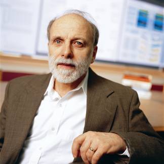
Prof. Stuart Rice, University of Chicago. He has done as much as anyone in a tremendous variety of theoretical studies including studies of interfaces and using coherent external perturbations to control chemical processes.
Not only can electronic wavefunctions tell us about the average
values of all physical properties for any particular state (i.e.,
yk above), but they also allow
us to tell how a specific "perturbation" (e.g., an electric field in
the Stark effect, a magnetic field in the Zeeman effect, light's
electromagnetic fields in spectroscopy) can alter the specific state
of interest. For example, the perturbation arising from the electric
field of a photon interacting with the electrons in a molecule is
given within the so-called electric dipole approximation (see, for
example, Simons and Nichols, Ch.
14) by:
Hpert =Sj e2 rj • E (t)
where E is the electric field
vector of the light, which depends on time t in an oscillatory
manner, and ri is the vector denoting the spatial
coordinates of the ith electron. This perturbation,
Hpert acting on an electronic state yk
can induce transitions to other states yk'
with probabilities that are proportional to the square of the
integral
Ú yk'* Hpert yk dr .
So, if this integral were to vanish, transitions between
yk and
yk' would not occur, and
would be referred to as "forbidden". Whether such integrals vanish or
not often is determined by symmetry. For example, if yk
were of odd symmetry under a plane of symmetry sv
of the molecule, while yk' were
even under sv , then the
integral would vanish unless one or more of the three cartesian
components of the dot product rj • E were odd under
sv The general idea is that for
the integral to not vanish the direct product of the symmetries of
yk and of yk'
must match the symmetry of at least one of the symmetry components
present in Hpert . Professor Poul
Jørgensen has been especially involved in developing
such so-called response theories for perturbations that may be time
dependent (e.g., as in the interaction of light's electromagnetic
radiation).
As a preamble to the following discussion, I wish to draw the
readers' attention to the web pages of several prominent theoretical
chemists who have made major contributions to the development and
applications of electronic structure theory and who have agreed to
allow me to cite them in this text. In addition to the people
specifically mentioned in this text for whom I have already provided
web links, I encourage you to look at the following web pages for
further information:
 |
Professor Ernest Davidson, Univ. of Washington and Indiana University has contributed as much as anyone both to the development of the fundamentals of electronic structure theory and its applications to many perplexing problems in molecular structure and spectroscopy. |
|
The late Professor John Pople, Northwestern University, made developments leading to the suite of Gaussian computer codes that now constitute the most widely used electronic structure computer programs.His contributions to theory were recognized in his sharing the 1998 Nobel Prize in Chemistry. |
|
 |
Professor Bill Goddard, Cal Tech. When most quantum chemists were pursuing improvements in the molecular orbital method, he returned to the valence bond theory and developed the so-called GVB methods that allow electron correlation to be included within a valence bond framework. |
|
Professor Fritz Schaefer, University of Georgia. He has carried out as many applications of modern electronic structure theory to important chemical problems as anyone. |
|
 |
Professor Rod Bartlett, University of Florida. He brought the coupled-cluster method, developed earlier by others, into the mainstream of electronic structure theory. |
Professor Bernd Heb, University of Erlangen, has a special focus in his research on relativistic effects and the development of tools needed to study them.
Professor Hans-Joachim Werner, University of Stuttgart, has for many years pioneered developments of multi-configurational SCF and coupled-cluster methods and applied them to a wide variety of chemical problems.

Professor David Bishop, University of Ottawa, says the following about his recent research efforts:
Precise calculations of electrical and magnetic properties of small molecules and atoms; nonlinear optical properties, Faraday effect, Kerr effect, Cotton-Mouton effect, second- and third-harmonic generation; the effect of electric fields on nuclear motion.

Professor David Bishop, University of Ottawa
Professor Sigrid Peyerimhoff, Bonn University, is one of the earliest pioneers of multi-reference configuration interaction methods and has applied these powerful tools to many important chemical species and reactions. She has prepared a wonderful web site that details much of the history of the development of quantum chemistry.
|
The late Professor Mike Zerner, University of Florida, was very influential in continuing the development of semi-empirical methods within quantum chemistry. Such methods can be applied to much larger molecules than ab initio methods, so their continued evolution is an essential component to growth in this field of theoretical chemistry. |
|
Professor Poul Jørgensen of Aarhus University
spent much of his early career developing the fundamentals of electron and polarization propagator theory. Following up on that early work, he moved on to develop the tools of response theory (time dependent and time independent) for computing a wide variety of molecular properties. His group has combined the power of response theory with several powerful wavefunctions including coupled-cluster and configuration interaction functions.
The full N-electron Schrödinger equation governing the
movement of the electrons in a molecule is
[-h2 /2me Si=1i2 - Sa Si Za e2 /ria + Si,j e2 /rij ] y = E y .
In this equation, i and j label the electrons and a labels the nuclei. Even at the time this material was written, this equation had been solved only for the case N=1 (i.e., for H, He+ , Li2+ , Be3+ , etc.). What makes the problem difficult to solve for other cases is the fact that the Coulomb potential e2/rij acting between pairs of electrons depends upon the coordinates of the two electrons ri and rj in a way that does not allow the separations of variables to be used to decompose this single 3N dimensional second-order differential equation into N separate 3-dimensional equations.
However, by approximating the full electron-electron
Coulomb potential Si,j e2
/rij by a sum of terms, each depending on the
coordinates of only one electron Si,
V(ri ), one arrives at a Schrödinger equation
[-h2 /2me Si=1
which is separable. That is, by assuming that
y (r1 , r2 , ... rN ) = f1 (r1 ) f2 (r2) ... fN (rN),
and inserting this ansatz into the approximate Schrödinger
equation, one obtains N separate Schrödinger equations:
[-h2 /2me
one for each of the N so-called orbitals fi whose energies Ei are called orbital energies.
It turns out that much of the effort going on in the electronic
structure area of theoretical chemistry has to do with how one can
find the "best" effective potential V(r); that is, the
V(r), which depends only on the coordinates r of one
electron, that can best approximate the true pairwise additive
Coulomb potential experienced by an electron due to the other
electrons. The simplest and most commonly used approximation for
V(r) is the so-called Hartree-Fock (HF) potential:
V(r) fi (r) = Sj [ Ú|fj (r')|2 e2 /|r-r'| dr' fi (r)
- Úfj*(r') fj (r') e2 /|r-r'| dr' fj (r) ].
This potential, when acting on the orbital fi
, can be viewed as multiplying fi
by a sum of potential energy terms (which is what makes it
one-electron additive), each of which consists of two parts:
a. An average Coulomb repulsion Ú
|fj (r')|2
e2 /|r-r'| dr' between the electron in
fi with another electron whose
spatial charge distribution is given by the probability of finding
this electron at location r' if it resides in orbital
fj : |fj
(r')|2 .
b. A so-called exchange interaction between the electron in
fi with the other electron that
resides in fj..
The sum shown above runs over all of the orbitals that are occupied in the atom or molecule.
For example, in a Carbon atom, the indices i and j run over the two 1s orbitals, the two 2s orbitals and the two 2p orbitals that have electrons in them (say 2px and 2py ) The potential felt by one of the 2s orbitals is obtained by setting fi = 2s, and summing j over j=1s, 1s, 2s, 2s, 2px , 2py . The term Ú |1s(r')|2 e2 /|r-r'| dr' 2s(r) gives the average Coulomb repulsion between an electron in the 2s orbital and one of the two 1s electrons; Ú |2px(r')|2 e2 /|r-r'| dr' 2s(r) gives the average repulsion between the electron in the 2px orbital and an electron in the 2s orbital; and Ú |2s(r')|2 e2 /|r-r'| dr' 2s(r) describes the Coulomb repulsion between one electron in the 2s orbital and the other electron in the 2s orbital. The exchange interactions, which arise because electrons are Fermion particles whose indistinguishability must be accounted for, have analogous interpretations.
For example, Ú 1s*(r') 2s(r') e2 /|r-r'| dr' 1s(r) is the exchange interaction between an electron in the 1s orbital and the 2s electron; Ú 2px*(r') 2s(r') e2 /|r-r'| dr' 2px(r) is the exchange interaction between an electron in the 2px orbital and the 2s electron; and Ú 2s*(r') 2s(r') e2 /|r-r'| dr' 2s(r) is the exchange interaction between a 2s orbital and itself (note that this interaction exactly cancels the corresponding Coulomb repulsion Ú |2s(r')|2 e2 /|r-r'| dr' 2s(r), so one electron does not repel itself in the Hartree-Fock model).
There are two primary deficiencies with the Hartree-Fock
approximation:
a. Even if the electrons were perfectly described by a wavefunction
y (r1 ,
r2 , ... rN ) = f1
(r1 ) f2
(r2) ... fN
(rN) in which each electron occupied an
independent orbital and remained in that orbital for all time, the
true interactions among the electrons Si,j
e2 /rij are not perfectly represented by
the sum of the average interactions.
b. The electrons in a real atom or molecule do not exist in
regions of space (this is what orbitals describe) for all time; there
are times during which they must move away from the regions of space
they occupy most of the time in order to avoid collisions with other
electrons. For this reason, we say that the motions of the electrons
are correlated (i.e., where one electron is at one instant of time
depends on where the other electrons are at that same time).
Let us consider the implications of each of these two
deficiencies.
To examine the difference between the true Coulomb repulsion between electrons and the Hartree-Fock potential between these same electrons, the figure shown below is useful. In this figure, which pertains to two 1s electrons in a Be atom, the nucleus is at the origin, and one of the electrons is placed at a distance from the nucleus equal to the maximum of the 1s orbital's radial probability density (near 0.13 Å). The radial coordinate of the second is plotted along the abscissa; this second electron is arbitrarily constrained to lie on the line connecting the nucleus and the first electron (along this direction, the inter-electronic interactions are largest). On the ordinate, there are two quantities plotted: (i) the Hartree-Fock (sometimes called the self-consistent field (SCF) potential) Ú |1s(r')|2 e2 /|r-r'| dr', and (ii) the so-called fluctuation potential (F), which is the true coulombic e2/|r-r'| interaction potential minus the SCF potential.
As a function of the inter-electron distance, the fluctuation
potential decays to zero more rapidly than does the SCF potential.
However, the magnitude of F is quite large and remains so over an
appreciable range of inter-electron distances. Hence, corrections to
the HF-SCF picture are quite large when measured in kcal/mole. For
example, the differences DE between the
true (state-of-the-art quantum chemical calculation) energies of
interaction among the four electrons in Be (a
and b denote the spin states of the
electrons) and the HF estimates of these interactions are given in
the table shown below in eV (1 eV = 23.06 kcal/mole).
|
|
|
|
|
|
|
|
|
|
|
|
|
|
|
|
These errors inherent to the HF model must be compared to the total (kinetic plus potential) energies for the Be electrons. The average value of the kinetic energy plus the Coulomb attraction to the Be nucleus plus the HF interaction potential for one of the 2s orbitals of Be with the three remaining electrons -15.4 eV; the corresponding value for the 1s orbital is (negative and) of even larger magnitude. The HF average Coulomb interaction between the two 2s orbitals of 1s22s2 Be is 5.95 eV. This data clearly shows that corrections to the HF model represent significant fractions of the inter-electron interaction energies (e.g., 1.234 eV compared to 5.95- 1.234 = 4.72 eV for the two 2s electrons of Be), and that the inter-electron interaction energies, in turn, constitute significant fractions of the total energy of each orbital (e.g., 5.95 -1.234 eV = 4.72 eV out of -15.4 eV for a 2s orbital of Be).
The task of describing the electronic states of atoms and molecules from first principles and in a chemically accurate manner (± 1 kcal/mole) is clearly quite formidable. The HF potential takes care of "most" of the interactions among the N electrons (which interact via long-range coulomb forces and whose dynamics requires the application of quantum physics and permutational symmetry). However, the residual fluctuation potential is large enough to cause significant corrections to the HF picture. This, in turn, necessitates the use of more sophisticated and computationally taxing techniques to reach the desired chemical accuracy.
What about the second deficiency of the HF orbital-based model? Electrons in atoms and molecules undergo dynamical motions in which their coulomb repulsions cause them to "avoid" one another at every instant of time, not only in the average-repulsion manner that the mean-field models embody. The inclusion of instantaneous spatial correlations among electrons is necessary to achieve a more accurate description of atomic and molecular electronic structure.
Some idea of how large the effects of electron correlation are and
how difficult they are to treat using even the most up-to-date
quantum chemistry computer codes was given above. Another way to see
the problem is offered in the figure shown below. Here we have
displayed on the ordinate, for Helium's 1S
(1s2) state, the probability of finding an electron whose
distance from the He nucleus is 0.13Å (the peak of the 1s
orbital's density) and whose angular coordinate relative to that of
the other electron is plotted on the absissa. The He nucleus is at
the origin and the second electron also has a radial coordinate of
0.13 Å. As the relative angular coordinate varies away from
0 deg, the electrons move apart; near 0
deg, the electrons approach one another. Since both electrons have
the same spin in this state, their mutual Coulomb repulsion alone
acts to keep them apart.
What this graph shows is that, for a highly accurate wavefunction
(one constructed using so-called Hylleraas functions that depend
explicitly on the coordinates of the two electrons as well as on
their interparticle distance coordinate) that is not of the simple
orbital product type, one finds a "cusp" in the probability density
for finding one electron in the neighborhood of another electron with
the same spin. The probability plot for the Hylleraas function is the
lower dark line in the above figure. In contrast, this same
probability density, when evaluated for an orbital-product
wavefunction (e.g., for the Hartree-Fock function) has no such cusp
because the probability density for finding one electron at r,
q, f is
independent of where the other electron is (due to the product nature
of the wavefunction). The Hartree-Fock probability, which is not even
displayed above, would thus, if plotted, be flat as a function of the
angle shown above. Finally, the graph shown above that lies above the
Hylleraas plot and that has no "sharp" cusp was extracted from a
configuration interaction wavefunction for He obtained using a rather
large correlation consistent polarized valence quadruple atomic basis
set. Even for such a sophisticated wavefunction (of the type used in
many state of the art ab initio calculations), the cusp in the
relative probability distribution is clearly not well
represented.
Although highly accurate methods do exist for handling the correlated motions of electrons (e.g., the Hylleraas method mentioned above), they have not proven to be sufficiently computationally practical to be of use on atoms and molecules containing more than a few electrons. Hence, it is common to find other methods employed in most chemical studies in which so-called correlated wavefunctions are used.
By far, the most common and widely used class of such
wavefunctions involve using linear combinations of orbital product
functions (actually, one must use so-called antisymmetrized orbital
products to properly account for the fact that Fermion wavefunctions
such as those describing electrons are odd under permutations of the
electrons' labels):
Y = S J CJ| fJ1 fJ2 fJ3 ...fJ(N-!) fJN |,
with the indices J1, J2, ..., JN labeling the spin-orbitals and
the coefficients CJ telling how much of each particular
orbital product to include. As an example, one could use
Y = C1 |1sa 1sb | - C2 [|2pza2pzb | - |2pxa2pxb | -2pya2pyb |]
as a wavefunction for the 1S state of He (the last three orbital products are combined to produce a state that is spherically symmetric and thus has L = 0 electronic angular momentum just as the |1sa1sb| state does).
Using a little algebra, and employing the fact that the orbital
products
|f1 f2 | = (2)-1/2 [ f1 f2 - f2 f1 ]
are really antisymmetric products, one can show that the above He
wavefunction can be rewritten as follows:
Y = C1/3 {|fz a f'z b| - |fx a f'xb| - |fya f'y b| },
where fz = 1s +
(3C2/C1)1/2 2pz and
f'z = 1s -
(3C2/C1)1/2 2pz , with
analogous definitions for fx ,
f'x , fy
, and f'y . The physical
interpretation of the three terms ({|fz
a f'z
b| , |fx
a f'x
b| , and |fy
a f'y
b| ) is that |fz
a f'z
b| describes a contribution to
Y in which one electron of a
spin resides in a region of space described by fz
while the other electron of b spin
is in a region of space described by f'z
, and analogously for |fxa
f'x b|
and |fy a
f'y b|.
Such a wavefunction thus allows the two electrons to occupy different
regions of space since each orbital f in a
pair is different from its partner f'. The
extent to which the orbital differ depends on the
C2/C1 ratio which, in turn, is governed by how
strong the mutual repulsions between the two electrons are. Such a
pair of so-called polarized orbitals is shown in the figure
below.
These approaches provide alternatives to the conventional tools of quantum chemistry. The CI, MCSCF, MPPT/MBPT, and CC methods move beyond the single-configuration picture by adding to the wave function more configurations whose amplitudes they each determine in their own way. This can lead to a very large number of CSFs in the correlated wave function, and, as a result, a need for extraordinary computer resources.
The density functional approaches are different. Here one solves a
set of orbital-level equations
[ -h2/2me
+ U(r)] fi = ei fi
in which the orbitals {fi} 'feel' potentials due to the nuclear centers (having charges ZA), Coulombic interaction with the total electron density r(r'), and a so-called exchange-correlation potential denoted U(r'). The particular electronic state for which the calculation is being performed is specified by forming a corresponding density r(r'). Before going further in describing how DFT calculations are carried out, let us examine the origins underlying this theory.
The so-called Hohenberg-Kohn theorem
states that the ground-state electron density r(r)
describing an N-electron system uniquely determines the potential
V(r) in the Hamiltonian
H = Sj {-h2/2me
and, because H determines the ground-state energy and wave
function of the system, the ground-state density r(r)
determines the ground-state properties of the system. The proof of
this theorem proceeds as follows:
a. r(r) determines N because Ú r(r) d3r = N.
b. Assume that there are two distinct potentials (aside from an additive constant that simply shifts the zero of total energy) V(r) and V'(r) which, when used in H and H', respectively, to solve for a ground state produce E0, Y (r) and E0', Y'(r) that have the same one-electron density: Ú |Y|2 dr2 dr3 ... drN = r(r)= Ú |Y'|2 dr2 dr3 ... drN .
c. If we think of Y' as trial variational wave function for the Hamiltonian H, we know that
E0 < <Y'|H|Y'> = <Y'|H'|Y'> + Ú r(r) [V(r) - V'(r)] d3r = E0' + Ú r(r) [V(r) - V'(r)] d3r.
d. Similarly, taking Y as a trial function for the H' Hamiltonian, one finds that
E0' < E0 + Ú r(r) [V'(r) - V(r)] d3r.
e. Adding the equations in c and d gives
E0 + E0' < E0 + E0',
a clear contradiction.
Hence, there cannot be two distinct potentials V and V' that give the same ground-state r(r). So, the ground-state density r(r) uniquely determines N and V, and thus H, and therefore Y and E0. Furthermore, because Y determines all properties of the ground state, then r(r), in principle, determines all such properties. This means that even the kinetic energy and the electron-electron interaction energy of the ground-state are determined by r(r). It is easy to see that Ú r(r) V(r) d3r = V[r] gives the average value of the electron-nuclear (plus any additional one-electron additive potential) interaction in terms of the ground-state density r(r), but how are the kinetic energy T[r] and the electron-electron interaction Vee[r] energy expressed in terms of r?
The main difficulty with DFT is that the Hohenberg-Kohn theorem shows that the ground-state values of T, Vee , V, etc. are all unique functionals of the ground-state r (i.e., that they can, in principle, be determined once r is given), but it does not tell us what these functional relations are.
To see how it might make sense that a property such as the kinetic energy, whose operator
-h2 /2me ![]() 2
involves derivatives, can be related to the electron density,
consider a simple system of N non-interacting electrons moving in a
three-dimensional cubic "box" potential. The energy states of such
electrons are known to be
2
involves derivatives, can be related to the electron density,
consider a simple system of N non-interacting electrons moving in a
three-dimensional cubic "box" potential. The energy states of such
electrons are known to be
E = (h2/2meL2) (nx2 + ny2 +nz2 ),
where L is the length of the box along the three axes, and nx
, ny , and nz are the quantum numbers
describing the state. We can view nx2 +
ny2 +nz2 = R2
as defining the squared radius of a sphere in three dimensions, and
we realize that the density of quantum states in this space is one
state per unit volume in the nx , ny , nz
space. Because nx , ny , and nz
must be positive integers, the volume covering all states with
energy less than or equal to a specified energy E =
(h2/2meL2) R2 is 1/8 the
volume of the sphere of radius R:
F(E) = 1/8 (4p/3) R3 = (p/6) (8meL2E/h2)3/2 .
Since there is one state per unit of such volume, F(E)
is also the number of states with energy less than or equal to E, and
is called the integrated density of states. The number of
states g(E) dE with energy between E and E+dE, the density of
states, is the derivative of F:
g(E) = dF/dE = (p/4) (8meL2/h2)3/2 E1/2 .
If we calculate the total energy for N electrons, with the states
having energies up to the so-called Fermi energy (i.e., the
energy of the highest occupied molecular orbital HOMO) doubly
occupied, we obtain the ground-state energy:
= (8p/5) (2me/h2)3/2 L3 EF5/2.
The total number of electrons N can be expressed as
N = 2g(e)dE= (8p/3) (2me/h2)3/2 L3 EF3/2,
which can be solved for EF in terms of N to then
express E0 in terms of N instead of EF:
E0 = (3h2/10me) (3/8p)2/3 L3 (N/L3)5/3 .
This gives the total energy, which is also the kinetic energy in this case because the potential energy is zero within the "box", in terms of the electron density r (x,y,z) = (N/L3). It therefore may be plausible to express kinetic energies in terms of electron densities r(r), but it is by no means clear how to do so for "real" atoms and molecules with electron-nuclear and electron-electron interactions operative.
In one of the earliest DFT models, the Thomas-Fermi theory,
the kinetic energy of an atom or molecule is approximated using the
above kind of treatment on a "local" level. That is, for each volume
element in r space, one assumes the expression given above to
be valid, and then one integrates over all r to compute the
total kinetic energy:
TTF[r] = Ú (3h2/10me) (3/8p)2/3 [r(r)]5/3 d3r = CF Ú [r(r)]5/3 d3r ,
where the last equality simply defines the CF constant
(which is 2.8712 in atomic units). Ignoring the correlation and
exchange contributions to the total energy, this T is combined with
the electron-nuclear V and Coulombic electron-electron potential
energies to give the Thomas-Fermi total energy:
E0,TF [r] = CF Ú [r(r)]5/3 d3r + Ú V(r) r(r) d3r + e2/2 Ú r(r) r(r')/|r-r'| d3r d3r',
This expression is an example of how E0 is given as a local density functional approximation (LDA). The term local means that the energy is given as a functional (i.e., a function of r) which depends only on r(r) at points in space but not on r(r) at more than one point in space.
Unfortunately, the Thomas-Fermi energy functional does not produce results that are of sufficiently high accuracy to be of great use in chemistry. What is missing in this theory are a. the exchange energy and b. the correlation energy; moreover, the kinetic energy is treated only in the approximate manner described.
In the book by Parr and Yang, it is
shown how Dirac was able to address the exchange energy for the
'uniform electron gas' (N Coulomb interacting electrons moving
in a uniform positive background charge whose magnitude balances the
charge of the N electrons). If the exact expression for the exchange
energy of the uniform electron gas is applied on a local level, one
obtains the commonly used Dirac local density approximation to the
exchange energy:
Eex,Dirac[r] = - Cx Ú [r(r)]4/3 d3r,
with Cx = (3/4) (3/p)1/3 = 0.7386 in atomic units. Adding this exchange energy to the Thomas-Fermi total energy E0,TF [r] gives the so-called Thomas-Fermi-Dirac (TFD) energy functional.
|
|
 |
|
|
|
|
Because electron densities vary rather strongly spatially near the
nuclei, corrections to the above approximations to T[r]
and Eex.Dirac are needed. One of the more commonly used
so-called gradient-corrected approximations is that invented
by Becke, and referred to as the
Becke88 exchange functional:
Eex(Becke88) = Eex,Dirac[r] -g Ú x2 r4/3 (1+6 g x sinh-1(x))-1 dr,
where x =r-4/3
|![]() r|,
and g is a parameter chosen so that the
above exchange energy can best reproduce the known exchange energies
of specific electronic states of the inert gas atoms (Becke finds
g to equal 0.0042). A common gradient
correction to the earlier T[r] is
called the Weizsacker correction and is given by
r|,
and g is a parameter chosen so that the
above exchange energy can best reproduce the known exchange energies
of specific electronic states of the inert gas atoms (Becke finds
g to equal 0.0042). A common gradient
correction to the earlier T[r] is
called the Weizsacker correction and is given by
dTWeizsacker = (1/72)(h/me) Ú |
Although the above discussion suggests how one might compute the
ground-state energy once the ground-state density r(r)
is given, one still needs to know how to obtain r.
Kohn and Sham (KS) introduced a set of so-called KS orbitals obeying
the following equation:
{-1/2
where the so-called exchange-correlation potential Uxc
(r) = dExc[r]/dr(r)
could be obtained by functional differentiation if the
exchange-correlation energy functional
Exc[r] were known. KS
also showed that the KS orbitals {fj}
could be used to compute the density r by
simply adding up the orbital densities multiplied by orbital
occupancies nj :
r(r) = Sj nj |fj(r)|2.
(here nj =0,1, or 2 is the occupation number of the orbital
fj in the state being studied)
and that the kinetic energy should be calculated as
T = Sj nj <fj(r)|-1/2
The same investigations of the idealized 'uniform electron gas'
that identified the Dirac exchange functional, found that the
correlation energy (per electron) could also be written exactly as a
function of the electron density r
of the system, but only in two limiting cases- the high-density limit
(large r) and the low-density limit. There
still exists no exact expression for the correlation energy even for
the uniform electron gas that is valid at arbitrary values of
r. Therefore, much work has been devoted
to creating efficient and accurate interpolation formulas connecting
the low- and high- density uniform electron gas expressions (see
Appendix E in the Parr and Wang book for further details). One such
expression is
EC[r] = Ú r(r) ec(r) dr,
where
ec(r) = A/2{ln(x/X) + 2b/Q tan-1(Q/(2x+b)) -bx0/X0 [ln((x-x0)2/X)
+2(b+2x0)/Q tan-1(Q/(2x+b))]
is the correlation energy per electron. Here x =
rs1/2 , X=x2 +bx+c, X0
=x02 +bx0+c and Q=(4c -
b2)1/2, A = 0.0621814, x0=
-0.409286, b = 13.0720, and c = 42.7198. The parameter rs
is how the density r enters since
4/3 prs3 is equal to
1/r; that is, rs is the radius
of a sphere whose volume is the effective volume occupied by one
electron. A reasonable approximation to the full
Exc[r] would contain
the Dirac (and perhaps gradient corrected) exchange functional plus
the above EC[r], but
there are many alternative approximations to the exchange-correlation
energy functional. Currently, many workers are doing their best to
"cook up" functionals for the correlation and exchange energies, but
no one has yet invented functionals that are so reliable that most
workers agree to use them.
To summarize, in implementing any DFT, one usually proceeds as follows:
1. An atomic orbital basis is chosen in terms of which the KS orbitals are to be expanded.
2. Some initial guess is made for the LCAO-KS expansion coefficients Cj,a: fj = Sa Cj,a ca.
3. The density is computed as r(r) = Sj nj |fj(r)|2 . Often, r(r) is expanded in an atomic orbital basis, which need not be the same as the basis used for the fj, and the expansion coefficients of r are computed in terms of those of the fj . It is also common to use an atomic orbital basis to expand r1/3(r) which, together with r, is needed to evaluate the exchange-correlation functional's contribution to E0.
4. The current iteration's density is used in the KS equations to determine the Hamiltonian
{-1/2 ![]() 2
+ V(r) + e2/2 Ú
r(r')/|r-r'|
dr' + Uxc(r) }whose "new" eigenfunctions
{fj} and eigenvalues
{ej} are found by solving the
KS equations.
2
+ V(r) + e2/2 Ú
r(r')/|r-r'|
dr' + Uxc(r) }whose "new" eigenfunctions
{fj} and eigenvalues
{ej} are found by solving the
KS equations.
5. These new fj are used to compute a new density, which, in turn, is used to solve a new set of KS equations. This process is continued until convergence is reached (i.e., until the fj used to determine the current iteration's r are the same fj that arise as solutions on the next iteration.
6. Once the converged r(r) is
determined, the energy can be computed using the earlier
expression
E [r] = Sj nj <fj(r)|-1/2
In closing this section, it should once again be emphasized that
this area is currently undergoing explosive growth and much scrutiny.
As a result, it is nearly certain that many of the specific
functionals discussed above will be replaced in the near future by
improved and more rigorously justified versions. It is also likely
that extensions of DFT to excited states (many workers are actively
pursuing this) will be placed on more solid ground and made
applicable to molecular systems. Because the computational effort
involved in these approaches scales much less strongly with basis set
size than for conventional (SCF, MCSCF, CI, etc.) methods, density
functional methods offer great promise and are likely to contribute
much to quantum chemistry in the next decade.
There is a nice DFT web site established by the Arias research group at Cornell devoted to a DFT project involving highly efficient computer implementation within object-oriented programming.
The development of electronic structure theory has been ongoing since the 1940s. At first, only a few scientists had access to computers, and they began to develop numerical methods for solving the requisite equations (e.g., the Hartree-Fock equations for orbitals and orbital energies, the configuration interaction equations for electronic state energies and wavefunctions). By the late 1960s, several research groups had developed reasonably efficient computer codes (written primarily in Fortran with selected subroutines that needed to run especially efficiently in machine language), and the explosive expansion of this discipline was underway. By the 1980s and through the 1990s, these electronic structure programs began to be used by practicing "bench chemists" both because they became easier to use and because their efficiency and the computers' speed grew (and cost dropped) to the point at which modest to large molecules could be studied at reasonable cost and effort.
Even with much faster computers, there remain severe bottlenecks to extending ab initio quantum chemistry tools to larger and larger molecules (and to extended systems such as polymers, solids, and surfaces). Two of the most difficult issues involve the two-electron integrals
(ci cj |1/r1,2| ck cl ). Nearly all correlated electronic structure methods express the electronic energy E (as well as its gradient and second derivative or Hessian) in terms of integrals taken over the molecular orbitals, not the basis atomic orbitals. This usually then requires that the integrals be first evaluated in terms of the basis orbitals and subsequently transformed from the basis orbital to the molecular orbital representation using the LCAO-MO expansion fj = Sa Cj,a ca. For example, one such step in the transformation involves computing
Sa Cj,a (ca cj |1/r1,2| ck cl ) = (fi cj |1/r1,2| ck cl ).
Four such one-index transformations must performed to eventually obtain the (fi fj |1/r1,2| fk fl ) integrals. Given a set of M basis orbitals, there are ca. M4/8 integrals (ca cj |1/r1,2| ck cl ). Each one-index transformation step requires ca. M5 calculations (i.e., to form the sum of products such as Sa Cj,a (ca cj |1/r1,2| ck cl ). Hence the task of forming these integrals over the molecular orbitals scales as the fifth power of M.
The research group of Professor Martin Head-Gordon has been attacking two aspects of the above integral bottleneck.

First, his group has been deriving and implementing in a very efficient manner expressions for the electronic energy (and its gradient with respect to nuclear positions ) that are not written in terms of integrals over the molecular orbitals but in terms of integrals over the basis atomic orbitals. This allows them to produce what are called "direct" procedures for evaluating energies and gradients. The advantages of such direct methods are (1) that one does not have to go through the M5 integral transformation process, and (2) that one does not have to first compute all of the atomic-orbital integrals (ci cj |1/r1,2| ck cl ). Instead, one can compute groups of these integrals (ci cj |1/r1,2| ck cl ) (e.g., as many as one can retain within the fast main memory of the computer), calculate the contributions made by these integrals to the energy or gradient, and then delete this group of integrals and proceed to compute (and use) another group of such integrals. This allows one to handle larger basis sets than when one has to first obtain all of the integrals and store them (e.g., on disk). The second major advance that the Head-Gordon group has fostered is developing clever and efficient new tools for computing the atomic-orbital-level two-electron integrals (ci cj |1/r1,2| ck cl ), especially when the product functions ci (1) cj (1) and ck (2) cl (2) invlove functions that are distant from one another. When there is good reason to view these products as residing in different regions of space (e.g., when the constitutent atomic orbitals are centered on atoms in different parts of a large molecule), so-called multipole expansion methods (and other tools) can be used to approximate the two-electron integrals (ci cj |1/r1,2| ck cl ). In this way, the Head-Gordon group has been able to (a) calculate integrals in which all of the basis orbitals reside on the same or very nearby atoms in conventional (highly efficient) ways, (b) approximate (very rapidly and in a numerically reliable multipolar manner) the integrals where the charge densities are somewhat distant yet still significant, and (c) ignore (to controlled tolerances) integrals for product densities that are even more distant. This has allowed them to obtain integral evaluation and energy-computation schemes that display nearly linear scaling with the number of atoms (and thus basis orbitals) in the system. It is only through such efforts that there is any hope of extending ab initio electronic structure mehtods to large molecules and extended systems.
The Head-Gordon group has also been expanding the horizons of the very powerful coupled-cluster method for treating electron correlation at a high level, especially by introducing so-called local-methods for handling interactions among electrons. In particular, by making clever defintions of localized occupied and virtual orbitals, they have been able to develop new methods whose computational effort promises to scale more practically with the number of electrons (i.e., the molecule size) than do conventional coupled cluster methods. Combining their advances in coupled-cluster theory with their breakthroughs in handling electron-electron interactions, has lead to a large body of important new work from this outstanding group.
At present, more electronic structure calculations are performed by non-theorists than by practicing theoretical chemists. This is largely due to the proliferation of widely used computer programs. This does not mean that all that needs to be done in electronic structure theory is done. The rates at which improvements are being made in the numerical algorithms used to solve the problems as well as at which new models are being created remain as high as ever. For example, Professor Rich Friesner has developed and Professor Emily Carter has implemented for correlated methods a highly efficient way to replace the list of two-electron integrals (fi fj |1/r1,2| fk fl ), which number N4 , where N is the number of atomic orbital basis functions, by a much smaller list (fi fj |l) from which the original integrals can be rewritten as: (fi fj |1/r1,2| fk fl ) = Sg (fi (g)fj (g)) Ú dr fk(r) fl (r)/|r-g| .
|
|
|
|
|
|
|
This tool, which they call pseudospectral methods, promises to reduce the CPU, memory, and disk storage requirements for many electronic structure calculations, thus permitting their applications to much larger molecular systems.
In addition to ongoing developments in the underlying theory and computer implementation, the range of phenomena and the kinds of physical properties that one needs electronic structure theory to address is growing rapidly. Professor Gustavo Scuseria has been especially active in developing new methods for treating very large molecules, in particular, methods whose computer requirements scale linearaly (or nearly so) with molecular size.
In addition, a great deal of progress has been made in constructing sequences of atomic orbital basis sets whose use allows one to extrapolate to essentially complete-basis quality results. Thom Dunning has, more than anyone else, been responsible for progress in this area.
 |
 |
|
|
|
|
There are a variety of tools that aim to compute differences betweeen state energies (e.g., electron affinities, ionization potentials, and excitation energies) directly. Several workers who have been instrumental in developing these methods include those shown below.
Professors Lorenz Cederbaum (l), University of Heidelberg, Professor Jan Linderberg (r), Aarhus University, and Professor Yngve Ohrn (below), University of Florida.
Also, Professor Howard Taylor, University of Southern California (below) contributed much to these developments as well as to methods for treating metastable electronic states.
In more recent years, the author, Professor J. V. Ortiz (below, l), Kansas State University, Professor P. Jørgensen (below, r), and Profesor J. Oddershede (bottom) have continued to develop these and related methods.
In addition to the many practicing quantum chemists introduced above, I show below photos of several others whose research and educational efforts will be of interest to students reading this web site.
 |
|
|
|
|

Professor Marcel Nooijen, University of Waterloo
At Yale University, Prof. Victor Batista is working on using quantum and semi-classical methods on many-molecule condensed-phase systems both in equilibrium and undergoing dynamical evolution. These systems inlcude biological species such as rhodopsin and semi-conductor materials.

Professor Victior S. Batista, Yale University
Professor Roi Baer, Hebrew University
Professor Baer is involved in a wide range of research at the interface between electronic structure and dynamics. He has a very nice web page devoted not only to his own group's efforts but detailing work of many other scholars.

Professor Krzysztof Szalewicz, Deleware
Professor Szalewicz has used so-called symmetry adapted perturbation theory (SAPT) to develop very accurate methods for evaluating weak intermolecular interactions. His group has also shown how to use such ideas to improve upon density functional theory by adding to DFT the effects of dispersion interactions which DFT usually leaves out.

Professor Millard Alexander, Maryland
Professor Alexander's group has contributed much to the study of the spectra, structure, and reactivity of molecular radicals, especially as influenced in collisions with other species.

Professor Kirk Peterson, Washington State University
Professor Peterson has been very active in developing systematic basis sets for use when employing correlated electronic structure methods. His web site offers a link to a wide range of such basis sets that can be downloaded in very convenient forms.
Professor John Herbert, Ohio State University
Professor John Herbert of Ohio State University is working on combined electronic and nuclear-motion dynamical studies of water cluster anions. His group is also involved in advancing the theoretical framework of photochemistry and developing novel and practical methods within electronic structure theory.
Professor Seymour Wang, Boston University
Professor Wang works on multi-scale Monte-Carlo simulations, the development of new force fields using force matching methods.

Professor Giulia Galli, Univ. of California, Davis
Professor Giulia Galli heads the ab initio nanoscience group at the Univ. of California, Davis.

Professor Sabre Kais, Purdue University

Professor Ramon Hernandez, Centro de Investigaciones Quimicas, Mexico
Professor Hernandez studies the effects of van der Waals complex formation or of bi-molecular collisions on the spectra and energetics and energy transfer within open-shell molecules.
Professor Kais describes his research as follows: The research in our group is mainly devoted to electronic structure and dynamics of atoms, molecules, clusters and quantum dots. The research program includes developing and applying the renormalization group, finite-size scaling and the pivot method.
Professor Alexei Stuchebrukhov, University of California, Davis
He describes his research as follows: We are interested in two fundamental processes in chemistry and biology: electron transfer and proton transfer. In our research we develop theory and perform large-scale computer simulations of these processes in complex biological molecular systems.
In addition to Prof. Balusubramanian, another expert on the effects of relativity on atomic and molecular properties is Prof. Pekka Pyykko of Helsinki University (below). This dynamic scholar always give a wonderful talk on how relativity contributes to many properties of matter in nature.


Professor Maciej Gutowski, Hariot-Watt University, Scotland
Professor Gutowski has been involved in a wide range of electronic stucture issues including dipole-bound electrons, electrons attaching to biological molecules, and the theory of intermolecular interactions.
Most people know that the study of transition metal containing systems is especially difficult because of the near-degeneracy of the ns and (n-1) d orbitals and the role of relativistic effects in the heavier elements. Prof. Gernot Frenking of the University of Marburg, shown below, has devoted a great deal of effort to understanding such systems. His group has also developed a powerful and useful means of decomposing the bonding interactions among atoms into various physical contributions.

Professor Gernot Frenking
Professor Piotr Piecuch, Michigan State University, has been involved in extending the coupled-cluster method to allow one to use multiconfigurational reference wave functions, which is very important when one wishes to describe diradicals and bond-breaking and bond-forming proceses. He and his co-workers have forumlated what they call a renormalized coupled-cluster method that can accurately describe bond breaking and excited electronic surfaces at a computational cost similar to that of a single-configuration reference calculation. They have also been looking into using explicitly correlated two-electron exponential cluster expansions of the N-electron wave function to see to what extent one can capture most (if not all) of the electron-electron correlations within such a compact framework.
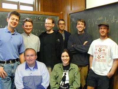
Professor Piotr Piecuch (upper left) with his research group at Michigan State Univesity

Professor Joe Francisco, Purdue University
Professor Francisco says of his research: Research in our laboratory focuses on basic studies in spectroscopy, kinetics and photochemistry of novel transient species in the gas phase.
Professor Nicholas Handy (above), Cambridge University, has made numerous contributions to electronic structure theory, to the theory of molecular spectroscopy, and to the rapidly expanding field of density functional theory.

Professor Jose Ramon Alvarez Collado (above) has made several contributions to Hartree-Fock and configuration interaction theory as well as to the treatment of vibtrational Hamiltonia and vibrational motions of molecules. He recently has shown how to handle large clusters or solid materials that contain a very large number of unpaired electrons.

Professor Andrew Rappe, University of Pennsylvania
Professor Rappe says of his research: My research group creates and uses new theoretical and computational approaches to study complex systems in materials science, condensed-matter physics, and physical chemistry.

Professor Thomas Sommerfeld, Southeast Louisina University
Professor Sommerfeld studies electron-driven chemistry, including electrons bound to water clusters and the metastable anion states that often arise when electrons bind weakly to molecules or molecular clusters.
 |
|
 |
|
|
|
|

Professor Bjørn Roos, Lund University, Sweden has been one of his nation's leading quantum chemists for many years, has developed one of the most powerful and widely used quantum chemistry codes, and has organized many schools on quantum chemistry.
Professor Jerzy Leszczynski at Jackson State University has established a very strong program in quantum chemistry and has hosted many very important conferences as well as "schools".
Professor Kimihiko Hirao's group in Tokyo has made many important contributions to the development and applications of modern quantum chemistry tools, especially those involving multi-configurational wave functions.

There exists an approach to solving the Schrödinger equation that has proven to be extremely accurate and is based on viewing the time-dependent Schrödinger equaiton as a diffusion equation with its time variable defined as imaginary. The idea then is to propagate an "initial" wavefunction (chosen to possess the proper permutational and symmetry properties of the desired solution) forward in time with the diffusion equation (having a source and sink term arising from the electron-nuclear and electron-electron Coulomb potentials). It can be shown that such a propogated wavefunction will converge to the lowest energy state that has the symmetry and nodal behavior of the trial wavefunction. The people who have done the most to propose, implement, and improve such so-called Diffusion Monte-Carlo type procedures include:
Professor Bill Lester, University of California, Berkeley
Professor Jules Moskowitz of New York University
and Professor David Ceperley of the University of Illinois
Professor Greg Gellene, Texas Tech, has pioneered the study of Rydberg species and of concerted reactions of small molecules and molcular compexes.

Professor Anna Krylov, University of Southern California, has been developing new electronic structure methods aimed at particularly difficult classes of compounds where multiconfigurational wave functions are essential. These include diradical and triradical species.

Professor Debbie Evans, University of New Mexico, has been working on electron transport and other quantum dynamics in branched macromolecules and other condensed phase systems.

Professor Angela Wilson, University of North Texas has done a lot to calibrate basis sets so we know to what extent we can trust them in various kinds of electronic structure calculations.

Prof. Angela Wilson
Professor Thomas Cundari, University of North Texas, is very active in using electronic structure methods to study inorganic and organometallic species.

Prof. Thomas Cundari (red shirt).
Professor Wes Borden recently joined the University of North Texas as Welch Professor. He has a long and distinguished record of applying quantum chemistry to important problems in organic chemistry.

Prof. Wes Borden
Professor Ludwik Adamowicz (below) of the University of Arizona has done a lot of work on molecular anions, especially
dipole-bound anions involving bio-molecules. He has also done much work on multi-reference coupled cluster methods,
method for generating non-adiabatic multiparticle wave functions, and for calculating rovibrational states of polyatomic molecules.
Many younger theoretical chemists are focusing efforts on simulating and understanding processes occurring in condensed media. One of the bright young stars in this direction is Professor Oleg Prezhdo at the University of Wisconsin in Seattle. The goal of Professor Prezhdo's research is to obtain a theoretical understanding at the molecular level of chemical reactivity and energy transfer in complex condensed-phase chemical and biological environments. This requires the development of new theoretical and computational tools and the application of these tools to challenging chemical problems in direct connection to experiments.
Professor Oleg Prezhdo, University of Washington (standing left at top)
Professor Kwang Kim, is using a variety of theoretical methods to study functional materials with the support of Creative Research Initiativ,
Ministry of Science and Technology of Korea. His laboratory has three subdivisions: (1) the quantum theoretical chemistry
group, (2) a theoretical condensed matter physics group, and (3)a synthesis and property measurement group.
Indiana University has had a long tradition of excellence in theoretical chemistry. Currently, its chemistry faculty include Prof. Peter Ortoleva, Prof. Krishnan Raghavachari, and Prof. Srinivasan Iyengar who are shown below.
Professor Peter Ortoleva who works on pattern formations within biological systems as well as in geology.

Professor Krishnan Raghavachari who has made numerous advances in quantum chemical methodologies and in the study of small to moderate size clusters of main group atoms.

Prof. Srinivasan Iyengar who developed the atom-centered density matrix propogation method for combining electronic structure and collision/reaction dynamics and is applying this to a wide variety of problems.
At Notre Dame University, there are also several faculty specializing in theory. They include

Prof. Eli Barkai who studies single-molecule spectroscopy and fractional kinetics.

Prof. Dan Gezelter who studies condensed-phase molecular dynamics, and

Prof. Dan Chipman who is interested in solvation effects, electronic structure methods developments and free radicals.
Several recent new faculty hires have been made in extremely good chemistry departments including those shown below. We need to be looking out for many good new developments from these people.

Prof. Garnet Chan, Cornell University, says the following about his group's work:
Our work is in the area of the electronic structure and dynamics of complex processes. We engage in developing new and more powerful theoretical techniques which enable us to describe strong electronic correlation problems.
Of particular theoretical interest are the construction of fast (polynomial) algorithms to solve the quantum many-particle problem, and the treatment of correlation in time-dependent processes.
A key feature of our theoretical approach is the use of modern renormalization group and multi-scale ideas. These enable us to extend the range of simulation from the simple to the complex, and from the small to the very large.
Some current phenomena under study include:
(i) Energy and electron transfer in conjugated polymers: specifically photosynthetic carotenoids, optoelectronic polymers, and carbon nanotubes,
(ii) Spin couplings in multiple-transition metal systems, including iron-sulfur proteins and molecular magnets.
(iii) Lattice models of high Tc superconductors.

Profesor Phillip Geissler, University of California, Berkeley

Professor Troy van Voorhis, MIT, says the following about his group's work:
The Van Voorhis group develops new methods that make reliable predictions about real systems for which existing techniques are inadequate. At present, our ideas center around the following major themes: the value of explicitly time-dependent theories, the importance of electron correlation and the proper treatment of delicate effects such as van der Waals forces and magnetic interactions.
Professor David Sherrill, Georgia Tech, has a strong research program focused on developing methods for properly describing the homolytic cleavage of chemical bonds and other cases in which more than a single Slater determinant become essential. He is also doing work on photochemistry, highly reactive species, and non-covalent interactions, all of which play central roles in many chemical processes.
Professor David Sherrill, Georgia Tech (above) and below with his group
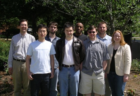
Sherrill research group as of 2005

Professor Robert Cave, Harvey Mudd College
Professor Cave shows that one can work at a high-quality primarily undergraduate institution and still be a major contributor. He has done some of the best work aimed at describing the mechanisms of electron transfer.

Profesor Jose Gascon, University of Connecticut
Professor Jose Gascon, University of Conecticut, is making use of combined quantum mechanics-molecular mechanics (QM-MM) approaches to study structure-function relations and biochemical reactivity of biomacromolecules.
Professor Ajit Thakkar, University of New Brunswick, has made many contributions to using quantum chemistry to study important chemical problems and has the following to say about his work:
My research concerns predictions of the properties of molecules and interactions between pairs of molecules. Such predictions are made using numerically-intensive computational methods based on quantum mechanics.

Professor Ajit Thakkar
At the University of Alberta, Prof.
P. N. Roy is working on the following:
Formal developments of the Feynman Path centroid approach for systems obeying Bose-Einstein statistics, Path Integral simulations of quantum fluids
* Simulations of doped helium nano-droplets
* Exact Quantum Dynamics of weakly bound clusters
* Molecular Dynamics simulation of Protein-ligand systems in solution and in the gas phase
* Dynamics of hydrogen bonded complexes and proton transfer
* Development of semi-classical quantum dynamics approaches
Professor P. N. Roy, Univ. of Alberta
Also at Georgia Tech is the reserach team of Prof. Rigoberto Hernandez, who focuses on a wide variety of scientific challenges in condensed-phase dynamics including protein folding, polymerization dynamics, and developing Langevin-type dynamics methods for use on non-stationary stochastic dynamical events.

Professor Rigoberto Hernandez, Georgia Tech.
Electronic Structure of Molecular Magnetism
Molecular magnetism is currently a ``hot'' area in chemical physics because of the technological promise of colossal magneto-resistant materials compounds and super-paramagnetic molecules. We are interested in developing a better fundamental understanding of magnetism that will allow us to predict the behavior of systems like these in an ab initio way. For example, one should be able to extract the Heisenberg exchange parameters (even for challenging oxo-bridged transition metal compounds) by simulating the response of the system to localized magnetic fields. We are also interested in extending the commonly used Heisenberg Hamiltonian to include spin orbit interactions in a local manner. This would be useful, for example, if one is interested in assembling a large molecule out of smaller building blocks - by knowing the preferred axis of each fragment one could potentially extract the magnetic axis and anisotropy of the larger compound.
Modeling Real-Time Electron Dynamics
Ab initio methods tend to focus the lion's share of attention on the description of electronic structure. However, there are a variety of systems where a focus on the electron dynamics is extremely fruitful. On the one hand, there are systems where it is the motion of the electrons that is interesting. This is true, for example, in conducting organic polymers and crystals - where it is charge migration that leads conductivity - and in photosynthetic and photovoltaic systems - where excited state energy transfer determines the efficiency. Also, in a very deep way, dynamic simulations can offer improved pictures of static phenomena. Here, our attention is focused on the fluctuation-dissipation theorem, an exact relation between the static correlation function and the time-dependent response of the system, and on semiclassical techniques, which provide a simple ansatz for approximating quantum results using essentially classical information.

Prof. Aaron Dinner, Univ. of Chicago
One of the leading figures in the field of determining small-molecule potential energy surfaces from spectroscopic and dynamics data is Professor Bob LeRoy of the University of Waterloo who says the following about his research efforts:
The determination and implications of intermolecular forces and the spectroscopy and dynamics of small molecules and molecular clusters. The development and application of methods for simulating and analysing photodissociation spectra of small molecules, and the discrete spectra of diatomic molecules and of polyatomic Van der Waals molecules, in order to determine the underlying potential energy surfaces. Simulations and predictions of dynamical properties and their spectroscopic signatures for chromophore molecules in molecular clusters of matrix environments.

Professor Boy LeRoy, University of Wateloo
Professor Dennis Salahub, University of Calgary, has contributed much to the development of modern density functional theory and tells us the following about his work:
His research group has improved Density Functional methods and software, which has helped to extend the range of applications. New improved functionals have been proposed, tested, and implemented in the code suite deMon, developed in Montreal and now in use in dozens of labs around the world. A fusion of DFT-deMon with other techniques (reaction fields, molecular dynamics, etc.) is underway. Current efforts are aimed at describing reactivity in complex environments: transition-metal catalysis, on the one hand, and enzymatic catalysis, on the other.

Professor Dennis Salahub, University of Calgary

Prof. Misha Ovchinnikov, Univ. of Rochester
Professor Jim Wright at Carleton University is carrying out electronic structure theory work on a variety of projects including the following in his words:
In my laboratory we use theoretical calculations to study chemical bonds in a variety of different environments. Part of the research is aimed at developing advances in theoretical methods, which can then be used to study important chemical properties such as the bond dissociation enthalpy, ionization potential, electron and proton affinity, hydrogen bond strengths and transition state energies.
Professor Jim Wright, Carleton University.
Prof. David Mazziotti, Univ. of Chicago
Professor Russell Boyd of Dalhouse University tells us the following about his research contributions, which are many:
Contemporary theoretical methods are used and developed to study a broad range of problems in chemistry, chemical physics and surface chemistry. Many projects involve collaboration with experimentalists and yield information which is unattainable by any other method.

Professor Russell Boyd, Dalhousie University
Professor Tom Ziegler at the University of Calgary has advanced the development and applications of density functional theory to a wide variety of important chemical and materials science problems including:
1. The optimization of transition state structures in elementary reaction steps of importance for homogeneous catalysis. Studies of the corresponding reaction paths by intrinsic reaction coordinates.
2. The dynamics of molecules chemisorped on metal surfaces.
3. The influence of relativity on the chemical bond and the periodicity of the elements.
4. First principle calculations of response properties such as frequencies, NMR and ESR parameters.
5. Modelling of steric bulk and solvation effects in elementary reaction steps.
6. Fundamental studies of density functional theory.
Professor Tom Ziegler, University of Calgary
Web page links to many of the more widely used programs offer convenient access:
Pacific Northwest Labs is developing a suite of programs called NWChem
The Gaussian suite of programs
The GAMESS program
The HyperChem programs of Hypercube, Inc.
The CAChe software packages from Fujitsu
The Spartan sofware package of Wavefunction, Inc.
The MOPAC program of CambridgeSoft
The Amber program of Prof. Peter Kollman, University of California, San Francisco
The CHARMm program
The programs of Accelrys, Inc.
The COLUMBUS program
The CADPAC program of Dr. Roger Amos
The programs of Wavefunction, Inc.
The ACES II program of Prof. Rod Bartlett.
The MOLCAS program of Prof. Bjorn Roos.
The MOLPRO quantum chemistry package of Profs. Werner and Knowles
The Vienna Ab Initio Simulations Package (VASP)
A nice compendium of various softwares is given in the Appendix of Reviews in Lipkowitz K B and Boyd D B (Eds) 1996 Computational Chemistry (New York, NY: VCH Publications) Vol 7
I hope the discussion I have offered has made it clear that there is every reason to believe that this sub-discipline of theoretical chemistry will continue to blossom for many years to come. Clearly, electronic structure theory provides a wealth of information about molecular structure and molecular properties. It does not, however, give us all the information we need to characterize a molecule's full motions. What is missing primarily is a description of the movements of the nuclei (or, equivalently, the bond lengths and angles and intermolecular coordinates), whose study lies within the realm of the next sub-discipline of theoretical chemistry to be discussed.
The collisions among molecules and resulting energy transfers
among translational, vibrational, rotational, and electronic modes,
as well as chemical reactions that occur intramolecularly or in
bi-molecular encounters lie within the realm of molecular and
chemical dynamics theory. The vibrational and rotational motions that
a molecule's nuclei undergo on any one of the potential energy
surfaces EkQ) is also a subject for molecular dynamics and
provides a logical bridge to the subject of molecular
vibration-rotation spectroscopy.
For any particular molecule with its electrons occupying one of its particular electronic states, the atomic centers (i.e., the N nuclei) undergo translational, rotational, and vibrational movements. The translational and rotational motions do not experience any forces and are thus "free motions" unless (1) surrounding solvent or lattice species are present or (2) an external electric or magnetic field is applied. Either of the latter influences will cause the translations and rotations to experience potential energies that depend on the location of the molecule's center of mass and the molecule's orientation in space, respectively.
In contrast, the vibrational coordinates of a molecule experience
forces that result from the dependence of the electronic state energy
Ek on the internal coordinates
Fi = - dEk({Q})/dQi.
By expressing the kinetic energy T for internal vibrational
motions and the corresponding potential energy V= Ek({Q})
in terms of 3N-6 internal coordinates {Qk}, classical
equations of motion based on the so-called Lagrangian L = T - V:
d/dt d[T-V]/di = d[T-V]/dQi
can be developed. If surrounding solvent species or external fields are present, equations of motion can also be developed for the three center of mass coordinates R and the three orientational coordinates W . To do so one must express the molecule-solvent intermolecular potential energy in terms of R and W, and the translational and orientational kinetic energies must also be written in terms of the time rates of change of R and W.
The equations of motion discussed above are classical. Most
molecular dynamics theory and simulations are performed in this
manner. When light atoms such as H, D, or He appear, it is often
essential to treat the equations of motion that describe their
motions (vibrations as well as translations and rotations in the
presence of solvent or lattice surroundings) using the
Schrödinger equation instead. This is a much more difficult
task.
Let us consider an example to illustrate the classical and quantum
treatments of dynamics. In particular, consider the collision of an
atom A with a diatomic molecule BC with all three atoms constrained
to lie in a plane.
Here the three atoms have a total of 2N = 6 coordinates because
they are constrained to lie in the X,Y plane. The center of mass of
the three atoms
x = (mA xA + mB xB + mC xC )/M
y = (mA yA + mB yB + mC yC )/M
requires two coordinates to specify, which leaves 2N-2 = 4
coordinates to describe the internal and overall orientational
arrangement of the three atoms. It is common (the reason will be
explained below) in such triatomic systems to choose the following
specific set of internal coordinates:
1. r, the distance between two of the atoms (usually the two that are bound in the A + BC collision);
2. R, the distance of the third atom (A) from the center of mass of the first two atoms (BC);
3. a and b ,
two angles between the r and R vectors and the
laboratory-fixed X axis, respectively.
In terms of these coordinates, the total energy (i.e., the
Hamiltonian) can be expressed as follows:
H = 1/2 m'2 + 1/2 m
2 + 1/2 m'R2
2 + 1/.2 m r2
2
+ 1/2 M (2 +
2 ) + V.
Here, m is the reduced mass of the BC
molecule (m =
mBmC/(mB +mc )) M is the
mass of the entire molecule M = mA + mB +
mC , and m' is the reduced mass of A relative to BC (m' =
mAmBC/(mA +mBC )). The
potential energy V is a function of R, r, and q
= a + b the
angle between the r and R vectors.
To eventually make a connection to the quantum mechanical
Hamiltonian, it is necessary to rewrite the above H in terms of the
coordinates and their so-called conjugate momenta. For any coordinate
Q, the conjugate momentum PQ is defined by
PQ =L/
For example,
PR = m'Pr = m
Pa = m' R2
Pb = m r2
allow H to be rewritten as
H = PR2/2m' + Pr2 /2m + Pa2 /2m'R2 + Pb2 /2mr2 + (PX2 + PY2 )/2M +V.
Because the potential V contains no dependence on X or Y, the center of mass motion (i.e., the kinetic energy (PX 2 + PY 2 )/2M) will time evolve in a straight-line trajectory with no change in its energy. As such, it can be removed from further consideration.
The total angular momentum of the three atoms about the Z- axis
can be expressed in terms of the four remaining coordinates as
follows:
LZ = m' R2
Since this total angular momentum is a conserved quantity (i.e.,
for each trajectory, the value of LZ remains unchanged
throughout the trajectory), one can substitute this expression for
Pa and rewrite H in
terms of only three coordinates and their momenta:
H = PR2 /2m' + pr2 /2m + (LZ -Pb )2 /2m'R2 + Pb2 /2mr2 +V.
Notice that Pb is the angular momentum of the BC molecule (Pb = m r2 db/dt).
From this Hamiltonian (or the Lagrangian L = T - V), one can
obtain, using d/dt d[T-V]/d![]() i
= d[T-V]/dQi , the equations of motion for the
three coordinates and three momenta:
i
= d[T-V]/dQi , the equations of motion for the
three coordinates and three momenta:
dPR /dt = ![]() L/
L/![]() R
= -
R
= -![]() V/
V/![]() R
- (LZ -Pb
)2 /m'R3 ,
R
- (LZ -Pb
)2 /m'R3 ,
dPr /dt = -![]() V/
V/![]() r
- Pb2
/mr3 ,
r
- Pb2
/mr3 ,
dPb /dt =
-![]() V/
V/![]() b
= -
b
= -![]() V/
V/![]() q
,
q
,
dR/dt = PR /m',
dr/dt = Pr /m ,
db/dt = Pb
/mr2 .
These six classical equations of motion that describe the time
evolution of r, R, b, PR ,
pr , and Pb can then
be solved numerically as discussed earlier. The choice of initial
values of the coordinates and momenta will depend on the conditions
in the A + BC collision that one wishes to simulate. For example, R
will be chosen as very large, and PR will be negative
(reflecting inward rather than outward relative motion) and with a
magnitude determined by the energy of the collision
PR2 /2m' = Ecoll.. If the
diatomic BC is initially in a particular vibrational state, say v,
the coordinate r will be chosen from a distribution of values given
as the square of the v-state's vibrational wavefunction |yv
(r)|2 . The value of pr can then be
determined within a sign from the energy ev
of the v state: pr2 /2m
+ VBC = ev , where
VBC is the BC molecule's potential energy as a function of
r. Finally, the angle b can be selected
from a random distribution within 0<b<2p,
and Pb would be
assigned a value determined by the rotational state of the BC
molecule at the start of the collision.
The solution of the above six coupled first order differential equations may seem like it presents a daunting task. This is, however, not at all the case given the speed of modern computers. For example, to propagate these six equations using time steps of dt = 10-15 sec (one must employ a time step that is smaller than the period of the fastest motion- in this case, probably the B-C vibrational period which can be ca. 10-14 sec) for a total time interval of one nanosecond Dt = 10-9 sec, would require of the order of 106 applications of the above six equations. If, for example, the evaluation of the forces or potential derivatives appearing in these equations requires approximately 100 floating point operations (FPO), this 1 nanosecond trajectory would require about 108 FPOs. On a 100 Mflop (Mflop means million floating point operations per sec) desktop workstation, this trajectory would require only one second to run!
You might wonder about how long trajectories on much larger
molecules would run. The number of coordinates and momenta involved
in any classical dynamics simulations is 3N-6. The evaluation of the
force on any one atom due to its interactions with other atoms
typically requires computer time proportional to the number of other
atoms (since potentials and thus forces are often pairwise additive).
In such cases, the number of FPOs would be approximately:
#FPO = 100 x (Dt/dt) x ((3N-6)/3) x (3N-7)/2,
where the (3N-6)/3 factor scales the number of coordinates and
momenta from 3 in the above example to the number for a general
molecule containing N atoms, and (3N-9)/2 scales the number of
"other" coordinates that enter into the force calculation for any
given coordinate. Thus, we expect #FPO to vary as
#FPO = 100 x (Dt/dt) x 3N2 /2
for large N. Thus a trajectory run for 1 ns with time steps of
10-15 sec on a large bio-molecule containing 1000 atoms
would require approximately
#FPO = 1.5 x 10¹⁴
operations. Even with a 100 Mflop computer, this trajectory would run for 1.5 x10⁶ sec (or ca. 17 days!).
For such large-molecule simulations, which are routinely carried
out these days, it is most common to "freeze" the movement of the
high frequency coordinates (e.g., the C-H bond stretching motions in
a large bio-molecule), so that longer time steps can be taken (e.g.,
this may allow one to take dt = 10-14
sec or longer). It is also common to ignore the forces produced
on any given atom by those atoms that are far removed from the given
atom. In this way, one can obtain a simulation whose FPO requirements
do not scale as N2 but as NxN', where N' is the number of
atoms close enough to produce significant forces. By making such
approximations, classical trajectory simulations on molecules (or
molecules with solvent species also present) containing 1000 or more
moving atoms can be carried out in a matter of a few minutes per
trajectory.
Let us consider a case in which the collision A + BC is followed from its initial conditions through a time at which the A atom has struck the BC molecule and been scattered so A and BC are now traveling away from one another. In such a situation, we speak of a non-reactive collision.
Alternatively, the A + BC collision may result in formation of AB
+ C, which, of course, corresponds to a chemically reactive
collision. In this case, to follow the trajectory toward its ultimate
conclusion, it is common to employ a different set of internal
coordinates than were used in the early part of the collision. In
particular, one changes to two new distance and two new angular
coordinates as shown below.

These coordinates are analogous to those used to describe A + BC and are: r the distance from C to the center of mass of AB, t the AB internuclear distance, and two angles (g and f) between the x- axis and t and r, respectively.
So, as the classical Newton equations are solved in a step-by-step manner, eventually one changes from solving the equations for the time evolution of R, r, a, and b and their momenta to solving the corresponding equations for r, t, f, and g and their conjugate momenta. Then, once the C atom is far enough away (and still moving outward) to declare the collision ended, one can interrogate its outcome. In particular, one can examine the vibrational and/or rotational energy content of the product (BC in the non-reactive case; AB in the reactive case) diatomic molecule, and one can compute the relative kinetic energy (e.g., 1/2 m' (dr/dt)2 in the reactive case) with which the product fragments are moving away from one another. It is through such interrogation that one extracts information from classical trajectory simulations.
Professor Barbara Garrison, Penn State University, has exploited such classical trajectory simulations to study reactions and energy transfer processes taking place when an atom, ion, or molecule impacts a surface that may undergo ablation as a result of the impact.

Professor Barbara Garrison, Penn State University.
Let us now consider the above A + BC collision dynamics simulation but from the point of view of the quantum mechanical Schrödinger equation. This is a much more difficult problem to treat. Why? Because instead of having to solve six coupled first order differential equations subject to specified initial conditions, one must solve one four-dimensional partial differential equation: Hy = E y, where
or one must propagate in time
y (R,r,a,b;t) = exp[-i Ht/h] y(R,r,a,b;t=0)
to find y at time t, given initial
conditions for y at t=0.
Specifying an initial wavefunction y(R,r,a,b;t=0)
is not the difficult part of this quantum simulation. One would
probably form the initial wavefunction as a product of a vibrational
function yv (r) appropriate for
the vth level of the BC molecule, a rotational
wavefunction exp(iPb
b) describing rotation of the BC
molecule, and a relative-motion wavefunction yR
(R) describing motion along the R- coordinate and a function
exp(iPaa) describing the
angular momentum of A relative to the center of mass of the BC
molecule :
y(R,r,a,b;t=0) = yv (r ) exp(iPb b) exp (iPa a) yR (R).
If, alternatively, the initial value of the total angular momentum
is specified, the relation
LZ = m' R2
can be used to eliminate the initial Pa and express it in terms of Lz and Pb .
The most likely way to describe a collision in which the A atom
begins at a position R0 along the R- axis and with a
relative collision momentum along this coordinate of - PR
0 is to use a so-called coherent wave packet
function (see Professor Rick
Heller):
yR (R) = exp (-iPR0 R/h) [2p <dR>2 ]-1/2 exp (-(R-R0 )2 /(4<dR>2 )).
Professor Rick Heller
Here, the parameter <dR>2
gives the uncertainty or "spread" along the R- degree of freedom for
this wavefunction, defined as the mean squared displacement away from
the average coordinate R0 , since it can be shown for the
above function that
Ú (R-R0)2 yR* (R) yR (R) R2 dR = <dR>2
and that
R0 = Ú R yR *(R) yR (R) R2 dR.
It can also be shown that the parameter PR0
is equal to the average value of the momentum along the R
coordinate:
Ú yR (R)*{- ih
and that the uncertainty in the momentum along the R
coordinate:
<dPR2> = Ú yR (R)*{- ih
is related to the uncertainty in the R-coordinate by
<dPR2> <dR2 > =h2/4.
Note that for these coherent state wavefunctions, the
uncertainties fulfill the general Heisenberg uncertainty criterion
for any coordinate Q and its conjugate momentum P:
<dP2> <dQ2> >h2/4
but have the smallest possible product of uncertainties. In this
sense, the coherent state function is the closest possible to a
classical description (where uncertainties are absent).
The difficult part of the propagation process involves applying
the time evolution operator exp (- iHt/h) to this
initial wavefunction. The most powerful tools for applying this
operator fall under the class of methods termed Feynman path-integral
methods (see the links to Professors Greg
Voth, Nancy
Makri, and Jim
Doll). However, let us first examine an approach that has
been used for a longer time, for example in the hands of Professors
George Schatz
and John
Light.
 |
 |
|
|
|
|
 |
 |
|
|
|
|
|
|
||
|
|
Several other first-rate theorists have contributed much to the field of molecular dynamics, including quantum dynamics and condensed-media processes. They include those shown below:

Professor Chi Mak, USC
Professor Benny Gerber, Univ. of California, Irvine
Professor Debbie Evans, University of New Mexico

Professor Craig Martens, Univ. of California, Irvine


Professor Zlatko Bacic, New York University
Professor Bacic has done much to advance the theoretical dynamical study of floppy molecules and molecular clusters using a variety of techniques including quantum Monte-Carlo and discrete variable representation expansions.

Professor Ann McCoy, Ohio State University

Professor Ron Elber, Cornell Universtiy

Professor David Wales, Cambridge University
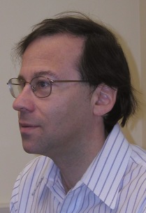
Professor Rob Coalson, University of Pittsburgh, one of the leaders in the applications of quantum dynamics to condensed phase and biological problems including ion channels.
If, alternatively, one prefers to attempt to solve the time-independent Schrödinger equation Hyk = Ek yk the most widely used approaches involve expanding the unknown y(R,r,a,b) in a basis consisting of products of functions of R, functions of r, and functions of a and of b:
yk = Sn,v,L,M Ck (n,v,L,M) Fn (R) yv(r) yL (b) yM (a).
This expansion is what one would use in the case of a non-reactive collision. If a chemical reaction (e.g., A + BC Æ AB + C) is to be examined, then one must add to the sum of terms given above another sum which contains products of functions of the so-called exit-channel coordinates (r, t, g, and f). In this case, one uses
yk = Sn,v,L,M Ck (n,v,L,M) Fn (R) yv(r) yL (b) yM (a)
+ Sn,v,L,M Ck (n,v,L,M) Fn (r) yv(t) yL (g) yM (f).
Of course, the yv , yL, Fn, and yM functions relating to the exit-channel are different than those for the entrance channel (e.g., yv (r) would be a AB-molecule vibrational wavefunction, but yv (r) would be a BC-molecule vibrational function).
As will be seen from the discussion to follow shortly, expanding
y in this manner and substituting into the
Schrödinger equation produces a matrix eigenvalue equation whose
eigenvalues are the Ek and the eigenvectors are the
expansion coefficients Ck (n,v,L,M). Given any
wavefunction y(R,r,a,b;t=0)
at t=0 (e.g., the one shown above may be appropriate for a collision
of A with a BC molecule in a specified vibrational/rotational state),
one can then express this wavefunction at later times as follows:
y(R,r,a,b;t) = Sk yk exp(-i Ekt/h) yk * y(R,r,a,b;t=0) dr .
This expression arises when one uses the facts that:
1. the {yk } form a complete set of functions so one can expand y(R,r,a,b;t=0) in this set, and
2. the time evolution operator exp (-i Ht/h) can
be applied to any eigenfunction yk
and produces exp (-i Ht/h) yk
= exp (-i Ekt/h) yk
.
So, it is possible to follow the time development of an initial
quantum wavefunction by first solving the time-independent
Schrödinger equation for all of the {yk
} and then expressing the initial wavefunction in
terms of the eigenfunctions (i.e, the integral Ú
yk * y(R,r,a,b;t=0)
dr is nothing but the expansion coefficient of y(R,r,a,b;t=0)
in terms of the yk ) after
which the wavefunction at a later time can be evaluated by the
expression
y(R,r,a,b;t) = Sk yk exp(-i Ekt/h) Ú yk * y(R,r,a,b;t=0) dr.
Let us now return to see how the expansion of y
in the manner
yk = Sn,v,L,M Ck (n,v,L,M) Fn (R) yv(r) yL (b) yM (a)
(or the generalization in which both entrance- and exit-channel
product functions are used) produces a matrix eigenvalue problem.
Substituting this expansion into Hy
=Ey and subsequently multiplying through
by the complex conjugate of one particular Fn' (R)
yv' (r) yL'
(b) yM'
(a)and integrating over R, r,
b, and a one
obtains a matrix eigenvalue equation:
H Ck = Ek Ck
in which the eigenvector is the vector of expansion coefficients
Ck (n.v,L,M) and the H matrix has elements
H(n,v,L,M|n',v',L',M')= < Fn' (R) yv' (r) yL' (b) yM' (a)| H | Fn (R) yv(r) yL (b) yM (a)>
given in terms of integrals over the basis functions with the
above Hamiltonian operator in the middle. Notice that in writing the
integral on the right-hand side of the above equation, the so-called
Dirac notation has been used. In this notation, any integral with a
wavefunction on the right, a complex conjugated wavefunction on the
left, and an operator in the middle is written as follows:
ÚY*Opfdq = < Y|Op|f>
What makes the solution of the four-variable Schrödinger
equation much more difficult than the propagation of the
four-coordinate (plus four-momenta) Newtonian equations? The
Hamiltonian differential operator
is non-separable because V depends on R, r, and q (which is related to b and a by q = a + b ) in a manner that can not be broken apart into an R-dependent piece plus an r-dependent piece plus a q-dependent piece. As a result, the four dimensional second-order partial differential equation can not be separated into four second-order ordinary differential equations. This is what makes its solution especially difficult.
To make progress solving the four-dimensional Schrödinger
equation on a computer, one is thus forced either to
1. expand y (R,r,a,b) as S C(n,v,L,M) Fn (R) yv(r) yL (b) yM (a), and then solve the resultant matrix eigenvalue problem, or to
2. represent y (R,r,a,b) on a grid of points in R, in r, and in a and b space and use finite-difference expressions (such as [F(R+dR) + F(R-dR) -2F(R)]/d2 to represent d2F(R)/dR2 ) to also express the derivatives on this same grid to ultimately produce a sparse matrix whose eigenvalues must be found.
In either case, one is left with the problem of finding eigenvalues of a large matrix. In, the former case, the dimension of the H matrix is equal to the product of the number of Fn (R) functions used in the expansion times the number of yv(r) functions used times the number of yL (b) used and times the number of yM (a) functions. In the latter case, the dimension of H is equal to the number of grid points along the R coordinate times the number of grid points along r times the number along b and times the number along a. It is the fact that the dimension of H grows quartically with the size of the basis or grid set used (because there are four coordinates in this problem; for a molecule with N atoms, the dimension of H would grow as the number of grid points or basis functions to the 3N-6 power!) and that the computer time needed to find all of the eigenvalues of a matrix grows as the cube of the dimension of the matrix (to find one eigenvalue requires time proportional to the square of the dimension) that makes the solution of this quantum problem very difficult.
Let us consider an example. Suppose that a grid of 100 points along the R-coordinate and 100 points along the r-coordinate were used along with say only 10 points along the a and b-coordinates. This would produce a (albeit very sparse) H matrix of dimension 106 . To find just one eigenvalue of such a large matrix on a 100 Mflop desktop workstation would require of the order of several times (106)2 /(100x106 ) sec, or at least 100 minutes. To find all 106 eigenvalues would require 106 times as long.
Given a wavefunction at t=0, y(R,r,a,b;t=0),
it is possible to propagate it forward in time using so-called path
integral techniques that Richard
Feynman pioneered and which have become more popular and
commonly used in recent years (see links to Professors Greg
Voth, Jim
Doll, and Nancy
Makri). In these approaches, one divides the time interval
between t=0 and t=t into N small increments of length t
= t/N, and then expresses the time evolution operator as a product of
N short-time evolution operators:
exp[-i Ht/h] = {exp[-i Ht/h]}N .
For each of the short time steps t ,
one then approximates the propagator as
exp[-i Ht/h] = exp[-i Vt/2h] exp[-i Tt/h] exp[-i Vt/2h],
where V and T are the potential and kinetic energy operators that appear in H = T + V. It is possible to show that the above approximation is valid up to terms of order t4 . So, for short times (i.e., small t ), these so-called symmetric split operator approximations to the propagator should be accurate.
The time evolved wavefunction y (t) can
then be expressed as
y (t) = { exp[-i Vt/2h] exp[-i Tt/h] exp[-i Vt/2h]}N y (t=0).
The potential V is (except when external magnetic fields are
present) a function only of the coordinates {qj } of the
system, while the kinetic term T is a function of the momenta
{pj } (assuming cartesian coordinates are used). By making
use of the completeness relations for eigenstates of the coordinate
operator
1 =dqj| qj> < qj|
and inserting this identity N times (once between each power of
exp[-i Vt/2h]
exp[-i Tt/h]
exp[-i Vt/2h]),
the expression given above for y (t) can
be rewritten as follows:
y (qN ,t)=exp{(-it/2
h)[V(qj) + V(qj-1)]}< qj| exp(-itT / h ) |qj-1>y (q0 ,0).
Then, by using the analogous completeness identity for the
momentum operator
1 = 1 / h
one can write
< qj| exp(-itT / h ) |qj-1> = 1 /hdp < qj|p > exp(-ip2t / 2mh) < p|qj-1 >.
Finally, by using the fact that the momentum eigenfunctions
|p>, when expressed as functions of coordinates q are given by
< qj|p > = (1/2p)1/2 exp(ipq/h),
the above integral becomes
< qj | exp(-itT /h) |qj-1> = 1/2 phh) exp[ip(qj - qj - 1)].
This integral over p can be carried out analytically to give
< qj | exp(-itT /h) |qj-1> =exp[im(qj - qj - 1)2 / 2
ht].
When substituted back into the multidimensional integral for
y (qN ,t), we obtain
y (qN ,t)=
h)[V(qj) + V(qj-1)]}
exp[im(qj - qj-1)2 /2ht] y (qo,0)
or
y (qN ,t) = ![]()
![]() dqN-1
dqN-2 . . . dq1 dq0
exp{i/
dqN-1
dqN-2 . . . dq1 dq0
exp{i/h ![]() [m(qj
- qj-1)2 / 2t
- t(V(qj)
+ V(qj-1))/2]} y (q0
, t=0).
[m(qj
- qj-1)2 / 2t
- t(V(qj)
+ V(qj-1))/2]} y (q0
, t=0).
Why are such quantities called path integrals? The sequence of positions q0 , q2 , ... qN describes a "path" connecting q0 to qN . By integrating over all of the intermediate positions q1 , q2 ,... qN-1 one is integrating over all such paths.
Further insight into the meaning of the above is gained by first
realizing that
(qj - qj-1)2 =
(qj - qj-1)2 t =
Tdt
is the representation, within the N discrete time steps of length
t, of the integral of Tdt over the
jth time step,
and that
[V(qj) + V(qj-1)] =
V(q)dt
is the representation of the integral of Vdt over the jth
time step. So, for any particular path (i.e., any specific set
of q0 , q1, , ... qN-1 , qN
values), the sum over all N such terms ![]() [m(qj
- qj-1)2 / 2t
- t(V(qj) +
V(qj-1))/2]
[m(qj
- qj-1)2 / 2t
- t(V(qj) +
V(qj-1))/2]
is the integral over all time from t=0 until t=t of the so-called
Lagrangian L = T - V:
[m(qj - qj-1)2 / 2t - t(V(qj) + V(qj-1))/2] =
Ldt.
This time integral of the Lagrangian is called the "action" S in
classical mechanics. Hence, the N-dimensional integral in terms of
which y (qN ,t) is expressed
can be written as
y (qN ,t) =exp{i /
hdt L } y (q0 ,t=0).
Here, the notation "all paths" is realized in the earlier version
of this equation by dividing the time axis from t=0 to t=t into N
equal divisions, and denoting the coordinates of the system at the
jth time step by qj . By then allowing each
qj to assume all possible values (i.e., integrating over
all possible values of qj ), one visits all possible paths
that begin at q0 at t=0 and end at qN at t=t.
By forming the classical action S
S = ![]() dtL
dtL
for each path and then summing exp(iS/h)
y ( q0 , t=0)
over all paths and multiplying by ![]() ,
,
one is able to form y (qN
,t).
![]() dqN-1
dqN-2 . . . dq1 dq0
exp{i/
dqN-1
dqN-2 . . . dq1 dq0
exp{i/h ![]() [m(qj
- qj-1)2 / 2t
- t(V(qj)
+ V(qj-1))/2]}
[m(qj
- qj-1)2 / 2t
- t(V(qj)
+ V(qj-1))/2]}
The difficult step in implementing this Feynman path integral method in practice involves how one identifies all paths connecting q0 , t=0 to qN , t. Each path contributes an additive term involving the complex exponential of the quantity
![]() [m(qj
- qj-1)2 / 2t
- t(V(qj) +
V(qj-1))/2]
[m(qj
- qj-1)2 / 2t
- t(V(qj) +
V(qj-1))/2]
This sum of many, many (actually, an infinite number) oscillatory
exp(iS/h) = cos (S/h) + i
sin(S/h) terms is extremely difficult to evaluate
because of the tendency of contributions from one path to cancel
those of another path. The evaluation of such sums remains a very
active research subject. The most commonly employed approximation to
this sum involves finding the path(s) for which the action
S= ![]() [m(qj
- qj-1)2 / 2t
- t(V(qj) +
V(qj-1))/2]
[m(qj
- qj-1)2 / 2t
- t(V(qj) +
V(qj-1))/2]
is smallest because such paths produce the lowest frequency
oscillations in exp(iS/h), and thus are not subject
to cancellation by contributions from other paths.
The path(s) that minimize the action S are, in fact the classical
paths. That is, they are the paths that the system whose quantum
wavefunction is being propagated in time would follow if the system
were undergoing classical Newtonian mechanics subject to the
conditions that the system be at q0 at t=0 and at qN
at t=t. In this so-called semi-classical approximation to the
propagation of the initial wavefunction using Feynman path integrals,
one finds all classical paths that connect q0 at t=0 and
at qN at t=t, and one evaluates the action S for each such
path. One then applies the formula
y (qN ,t) =h
but includes in the sum only the contribution from the classical path(s). In this way, one obtains an approximate quantum propagated wavefunction via a procedure that requires knowledge of only classical propagation paths.
Once an initial quantum wavefunction has been propagated for a time long enough for the event of interest to have occurred (e.g., long enough for an A + BC Æ AB + C reactive collision to take place in the above example problem), one needs to interpret the wavefunction in terms of functions that are applicable to the final-state. In the example considered here, this means interpreting y(R, r, a, b; t) in terms of exit-channel basis states that describe an intact AB molecule with a C atom moving away from it (i.e., the terms Sn,v,L,M Ck (n,v,L,M) Fn (r) yv(t) yL (g) yM (f)).
As explained earlier when the classical trajectory approach was
treated, to describe this final-state configuration of the three
atoms, one uses different coordinates than R,r,a,b
that were used for the initial state. The appropriate coordinates are
shown below in the figure.
That is, one projects the long-time wavefunction
y(R,r,a,b;t) = Sk yk exp(-i Ekt/h) Ú yk * y(R,r,a,b;t=0) dr
onto a particular exit-channel product function Fn
(r) yv(t)
yL (g)
yM (f)
to obtain the amplitude A of that exit channel in the final
wavefunction:
A = < Fn (r) yv(t) yL (g) yM (f)| y(R,r,a,b;t)>
= Sk < Fn (r) yv(t) yL (g) yM (f)| yk> exp(-iEkt/h) Ú yk * y(R,r,a,b;t=0) dr.
Using the earlier expansion for yk
, one sees that
< Fn (r) yv(t) yL (g) yM (f)| yk> = Ck (n,v,L,M)
for the exit channel, so the modulus squared of A, which gives the probability of finding the AB + C system in the particular final state
Fn (r) yv(t)
yL (g)
yM (f),
is given by:
|A|2 = | Sk Ck (n,v,L,M) exp(-i Ekt/h) Ú yk * y(R,r,a,b;t=0) dr |2 .
This result can be interpreted as saying that the probability of
finding the state Fn (r)
yv(t)
yL (g)
yM (f)
is computed by (1) first, evaluating the projection of the
initial wavefunction along each eigenstate (these components
are the Ú yk *
y(R,r,a,b;t=0)
dr), (2) multiplying by the projection of the specified
final wavefunction along each eigenstate (the < Fn
(r) yv(t)
yL (g)
yM (f)|
yk> = Ck
(n,v,L,M)), (3) multiplying by a complex phase factor exp(-i
h Ek t) that details how each eigenstate
evolves in time, and (4) summing all such products after which (5)
taking the modulus squared of the entire sum.
In addition to the people specifically mentioned in this text for
whom I have already provided web links, I encourage you to look at
the following web pages for further information:
|
|
Professor Bill Reinhardt, University of Washington. His early career focused on developing theories and computational tools for studying the dynamical decay of metastable states (e.g., such as occurs in unimolecular decomposition of molecules) and the rates of energy transfer among modes in molecules. |
|
Professor Richard Stratt, Brown University. He has been involved in examining the dynamics of clusters of atoms or molecules that are small on a macroscopic level (i.e., do not contain enough atoms to be considered to follow macroscopic thermodynamic laws) yet large enough to show certain characteristics (e.g., phase transition like behavior) associated with macroscopic systems. |
|
|
|
The late Professor Kent Wilson, University of California, San Diego. He was active in simulating dynamical behavior of a wide variety of complicated chemical and physical systems. His web sites contain some of the more "exciting" depictions and animations of molecular phenomena. |
|
Professor John
Tully, Yale University, has pioneered much of the
study of dynamics and reactions that occur at or near
surfaces and he invented the most commonly used so-called
surface hopping model for treating non-adiabatic transitions
among potential energy surfaces. |
|
Professor Mark Child, Oxford University has, along with Professor Bill Miller, Berkeley, developed the area of semi-classical collision and reaction dynamics. This approch to solving quantum equations in a manner that allows one to retain a great deal of classical mechanics' conceptual clarity has been very successufl and has lead to many new insights.

Professor Mark Child of Oxford University
Professor Bill Miller of Berkeley
Professor Don Truhlar, University of Minnesota was able to extend the Eyring idea of the transition state (the "pass" or col separating reactant and product valleys on the potential energy surface) by introducing what is now termed Variational Transition State Theory in which a pass on a free energy surface replaces the conventional transition state. He and his long-time collaborator, Dr. Bruce Garrett, succeeded in making this theory one of the most useful computational and conceptual tools in reaction dynamics.


Professor D avid Clary, University College, London has extended the capability of quantum reactive dynamics theory to systems with several degrees of freedom by introducing clever approximations that focus attention on certain "active" coordinates while treating other coordinates in an approximate manner. Such approaches are essential if one hopes to employ quantum methods on more than the simplest chemical reactions.

Professor Bob Wyatt, University of Texas,
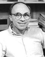
has played a primary role in developing new methods and algorithms that allow one to use quantum dynamics efficiently to study chemical reactions and energy flow in molecules and in collsions.

Professor Susan Tucker, University of California, Davis.

Professor Ned Sibert, University of Wisconsin, has been studing intramolecular energy flow and the interactions of lasers with small molecules. The goal of much of this work is to determine how one might control where the energy goes in a molecule that is photo-excited. This very exciting branch of photochemistry is eventually aimed at trying to control the energy (i.e., to keep it in certain internal modes) so that one might effect the outcome (i.e., which products are formed) of chemical reactions.
The University of Wisconsin, Madison has one of the longest traditions of excellence in theoretical chemistry, dating back to when the late Prof. Joseph O. Hirschfelder started the theortical chemistry institute (TCI). Their strength in theory continues to this day with Profs. Jim Skinner, Prof. Ned Sibert, Prof. John Harriman, Prof. Frank Weinhold, Prof. Arun Yethiraj, and Prof. Qiang Cui shown below.

Qiang Cui (left), whose works focus on macromolecules such as catalysis in enzymes or ATP hydrolysis in motor proteins, and John Harriman (right) whose efforts have emphasized gaining a better understanding of the electronic structure of molecules by use of reduced density matrices.


Professor Jim Skinner (left) whose work is discussed elsewhere and who serves as Director of TCI, Prof. Frank Weinhold (center) who invented the Natural Bond Orbital (NBO) analysis methods that offer a mathematically rigorous "Lewis structure" representation of the wavefunction, and Prof. Arun Yethiraj, who has contributed much to the statistical mechanical study of polyme materials.
Professor John Straub, Boston University is currently the Chair of the Theoretical Chemistry Subdivision of the Physical Chemistry Division of ACS. His work involves using molecular dynamics and Monte-Carlo simulation tools to study biomolecules, liquids, and clusters.
Two of John's colleagues at Boston University are

Professor David Coker whose group develops new methods for treating condensed-phase chemical dynamics and

Professor Tom Keyes whose group specializes in statistical mechanics of supercooled liquids
a. Large Biomolecules and Polymers
Following the motions of large molecules even using classical Newton equations involves special challenges. First, there is the fact that large molecules contain more atoms, so the Newtonian equations that must be solved involve many coordinates (N) and momenta. Because the potential energy functions,and thus the Newtonian forces, depend on the relative positions of the atoms, of which there are N(N-1)/2 , the computer time needed to carry out a classical trajectory varies as (at least) the square of the number of atoms in the molecule. Moreover, to adequately sample an ensemble of initial coordinates and momenta appropriate to a large molecule, one needs to run many trajectories. That is, one needs to choose a range initial values for each of the molecule's internal coordinates and momenta; the number of such choices is proportional to N. The net result is that computer time proportional to N3 (or worse) is needed,and this becomes a major challenge for large biomolecules or polymers. One way this problem is being addressed is to use parallel computers which allow one to run trajectories with different initial conditions on different processors.
Another problem that is special to large molecules involves the force field itself (see, for example, the web pages of Professors Andy McCammon, Charles Brooks and the late Peter Kollman, as well as of Biosym and CHARMm). Usually, the potential energy is expressed as a sum of terms involving:
1. bond stretching potentials of either harmonic V(r) = 1/2 k (r-re)2 or Morse form V(r) = De (1-exp(-b(r-re)))2
2. bond angle bending potentials of harmonic form depending on the angles between any three atoms A, B, C that are bonded to one another (e.g., the H-C-H angles in -CH2 - groups)
3. dihedral angles (e.g., the H-C-C-H angle in -H2C-CH2- groups
4. Van der Waals interactions V(r) = Ar-12 - Br-6 among all pairs of atoms (these potentials allow for repulsions among, for example, the H atoms of a methyl group in H3C-CH2-CH2-CH2-CH2-C H3 to repel the other H atoms as this "floppy" molecule moves into geometries that bring such groups into strong steric interaction)
5. electrostatic attraction (for opposite charges) and repulsions (for like charges) among charged or highly polar groups (e.g., between pairs of phosphate groups in a biopolymer, between a Na+ ion and a phosphate group, or between a charged group and a neighboring H2O molecule)
6. polarization of the electronic clouds of the large solute molecule or of surrounding solvent molecules induced by ionic or highly polar groups approaching highly polarizable parts of the molecule.
|
|
 |
|
|
|
|
Professor Charles Brooks
Professor Joan-Emma Shea, University of California, Santa Barbara, has been studying bio-molecules folding and motions as well.

Professor Joan Shea, University of California, Santa Barbara
Professor Frank Brown, also at Santa Barbara, says the following about his research:
Our interests lie in developing theoretical and computational tools from the physical sciences for use in studies of cellular biology. Currently we are pursuing three topics related to cellular functioning: membrane dynamics, cytoskeletal assembly and the kinetics of enzymatic turnover.

Professor Frank Brown, University of California, Santa Barbara
Professor Klaus Schulten (below) University of Illinois Physics, has studied many problems in biophysics. Most recently, he has focued
on the structure and function of supramolecular systems in the living cell, and on the development of non-equilibrium statistical mechanica
descriptions and efficient computing tools for structural biology.

Professor Zan Luthey-Schulten, University of Illinois Chemistry is one of the world's leading figures in using statistical mechancis techniques
to predict protein structures and to understand their relations to their functions.

One of the earliest pioneers in applying fundamental statistical mechanics, molecular mechanics, and solvation modelling theories to bio-molecules is Professor Arieh Warshel (below). His groups more recent interests include the dynamics of photobiological processes, enzyme catalysis and protein action, as well as the study of basic chemical reactions in solutions.
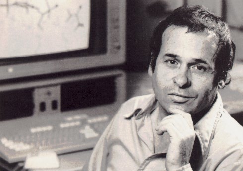
Professor Arieh Warshel, University of Southern Califonia

Professor Jeffry Madura, Duquesne Universtiy
The primary difficulties in using such a multi-parameterized force field are
1. that the values of the parameters characterizing each kind of potential have to be obtained either by requiring the results of a simulation to "fit" some experimental data or by extracting these parameters from ab initio quantum chemical calculations of the interaction potentials on model systems;
2. these developments and calibrations of the parameters in such force fields are still undergoing modifications and improvements, so they are not yet well established for a wide range of functional groups, solvents, ionic strengths, etc.
One more difficulty that troubles most large molecule simulations
is the wide range of time scales that must be treated when solving
the Newton equations. For example, in attempting to monitor the
uncoiling of a large biomolecule, which may occur over a time scale
of ca. 10-5 to 1 sec, one is usually forced to "freeze"
the much faster motions that occur (i.e., to treat the C-H, O-H, and
N-H bonds, which oscillate over ca.10-14 sec, as rigid).
If one were to attempt to follow the faster motions, one would have
to take time steps in solving the Newton equations of ca. 10-14
sec, as a result of which the uncoiling event would require
109 to 1014 time steps. Even with a computer
that could perform 109 floating point operations per
second (i.e., a one gigaflop computer), and assuming that a single
time step would use at least 1000 floating point operations (which is
very optimistic), a single such trajectory would use 103
to 108 seconds of computer time. This is simply
unrealistic. As a result, one is forced to freeze (i.e., by
constraining to fixed geometries) the faster motions so that the
Newton equations can be solved only for the slower motions. It is an
area of current research development to invent new methods that allow
such multiple time scale issues to be handled in a more efficient and
accurate manner.
One of the most pressing issues in chemical reaction dynamics involves how to treat a very large molecular system that is undergoing a chemical reaction or a photochemical event (i.e., a change that affects its electronic structure). Because the system's bonding and other attributes of its electronic wavefunction are changing during such a process, one is required to use quantum mechanical methods. However, such methods are simply impractical (because their computer time, memory, and disk space needs scale as the number of electrons in the system to the fourth (or higher) power) to use on very large molecules.
If the chemical reaction and/or photon excitation is localized
within a small portion of the molecular system (that may involve
solvent molecules too), there are so-called quantum
mechanics/molecular mechanics (QMMM) methods currently under much
development that can be employed. In these methods, one uses an
explicit quantum chemical (ab initio or semi-empirical) method
to handle that part of the system that is involved in the electronic
process. For example, in treating the tautomerization of
formamide H2 N-CHO to formamidic acid HN=CHOH in
aqueous solution,
one must treat the six atoms in the formamide explicitly using
quantum chemistry tools. The surrounding water molecules
(H2O)n could then be handled using a classical
force field (i.e., the formamide-water and water-water interaction
potentials as well as the internal potential energy function of each
H2O molecule could be expressed as a classical potential
like those described earlier in this section). If, on the other hand,
one wished to treat one or more of the H2O solvent
molecules as actively involved in promoting the tautomerization (as
shown in the figure below)
one would use quantum chemistry tools to handle the formamide plus the actively involved water molecule(s), and use classical potentials to describe the interactions of the remaining solvent molecules with these active species and among one another. At present, much effort is being devoted to developing efficient and accurate ways to combine quantum treatment of part of the system with classical treatment of the remainder of the system. Professor Chris Cramer has been very active developing new ways to model the influence of surrounding solvent molecules on chemical species whose spectroscopy or reactions one wishes to study.

Professors Mark Gordon, Than h Truong, Weito Yang, and Keji Morokuma are especially active in developing this kind of QMMM methods. Professor Truong has made some of his programs that compute rates of chemical reactions available through a web site called TheRate.
 |
 |
|
|
|
|

Professor Keiji Morokuma
As discussed earlier, it is often important to treat the electronic degrees of freedom, at least for the electrons involved in a chemical reaction or in a photon absorption or emission event, at a quantum level while still, at least for practical reasons, treating the time evolution of the nuclei classically. A novel approach developed by Car and Parrinello, and reviewed very nicely by Remler and Madden, incorporates the task of optimizing the electronic wavefunction into the Newtonian dynamics equations used to follow the nuclear movements.
The LCAO-MO coefficients Ci,k relating molecular
orbital fi to atomic orbital
ck are assumed to minimize an
energy function E[{Ci,k}] which can be a
Hartree-Fock or DFT-type function, for example. At each time step
during which the Newtonian equations
ma d2Xa /dt2 = -
are propagated, a corresponding propagation equation is used to follow the time evolution of the {Ci,k } coefficients. The latter equation was put forth by Car and Parrinello by defining a (fictitious) kinetic energy
T = Si, k 1/2 m |dCi,k/dt|2
in which the time derivatives of the Ci,k coefficients are viewed as analogs to the time rate of changes of the molecule's Cartesian coordinates {Xa}, and m is a (fictitious mass introduced to give this expression the units of energy. Then, using the dependence of the electronic energy E on the {Ci,k } to define the potential energy
V = E[{Ci,k}],
and then introducing a (fictitious) Lagrangian L = T-V whose classical action S = Ú L dt is made stationary with respect to variations in the {Ci,k } coefficients but subject to the constraint that the orbitals {fi} remain orthonormal:
di,j = S k,l C*i,k Sk,l Cj,l
the following dynamical equations are obtained for the Ci,k coefficients:
m d2Ci,k /dt2 = -
The left hand side of this equation gives the mass m multiplied by the "acceleration" of the Ci,k variable. The right side gives the "force" -
(since E[{Ci,k }] is made stationary with no constraint of orthogonality to lower-energy states) and one must realize that finite-time-step propagations with non-zero m render the {Ci,k} amplitudes obtained via classical propagation not equivalent to those obtained by minimizing E at each geometry.
Before closing this section on dynamics, I wish to bring to the readers' attention several other leading researchers in this exciting area of theoretical chemistry by showing photos of them below.
Professor Joel Bowman Emory University
Profess or Greg Ezra Cornell University
Professor Sharon Hammes-Schiffer Penn State University. Sharon's group has made use of basis set expansion approaches to follow the quantum dynamics of light nuclei such as H and D, and has applied this novel technique to a wide variety of biological and condensed-phase systems. Professor Jan Linderberg, Aarhus University
Dr. Steven Klippenstein,Sandia National Labs Pro fessor Chi Mak, University of Southern California
Professor Shaul Mukamel University of California, Irvine Professor Dan Neuhauser, UCLA C. Statistical mechanics provides the framework for studying large collections of molecules and tells us how to average over positions and velocities to properly simulate the laboratory distribution of molecules
When dealing with a sample containing a large number (e.g., billions) of molecules, it is impractical to attempt to monitor the time evolution of the coordinates and momenta (or analogous quantum state populations) of the individual constituent molecules. Especially for systems at or near equilibrium, these properties of individual molecules may vary irregularly on very short time scales (as the molecules undergo frequent collisions with neighbors), but the average behavior (e.g, average translational energy or average population of a particular vibrational energy level) changes much more gently with time. Such average properties can be viewed as averages for any one molecule over a time interval during which many collisions occur or as averages over all the molecules in the sample at any specific time.
By focusing on the most probable distribution of the total energy available to a sample containing many molecules and by asking questions that relate to the average properties of the molecules, the discipline of statistical mechanics provides a very efficient and powerful set of tools (i.e., equations) for predicting and simulating the properties of such systems. In a sense, the machinery of statistical mechanics allow one to describe the "most frequent" behavior of large molecular systems; that is how the molecules are moving and interacting most of the time. Fluctuations away from this most probable behavior can also be handled as long as these fluctuations are small.
1. The framework of statistical mechanics provides efficient equations for computing thermodynamic properties from molecular properties
a. The Boltzmann population equation
The primary outcome of asking what is the most probable distribution of energy among a large number N of molecules within a container of volume V that is maintained at a specified temperature T is the most important equation in statistical mechanics, the Boltzmann population formula:
Pj = Wj exp(- Ej /kT)/Q,
where Ej is the energy of the jth quantum state of the system (which is the whole collection of N molecules), T is the temperature in K, Wj is the degeneracy of the jth state, and the denominator Q is the so-called partition function:
Q = Sj Wj exp(- Ej /kT).
The classical mechanical equivalent of the above quantum Boltzmann population formula for a system with M coordinates (collectively denoted q and M momenta denoted p) is:
P(q,p) = h-M exp (- H(q, p)/kT)/Q,
where H is the classical Hamiltonian, and the partition function Q is
Q = h-M Ú exp (- H(q, p)/kT) dq dp .
b. The limit for systems containing many molecules
Notice that the Boltzmann formula does not say that only those states of a given energy can be populated; it gives non-zero probabilities for populating all states from the lowest to the highest. However, it does say that states of higher energy Ej are disfavored by the exp (- Ej /kT) factor, but if states of higher energy have larger degeneracies Wj (which they usually do), the overall population of such states may not be low. That is, there is a competition between state degeneracy, which tends to grow as the state's energy grows, and exp (-Ej /kT) which decreases with increasing energy. If the number of particles N is huge, the degeneracy W grows as a high power (say M) of E because the degeneracy is related to the number of ways the energy can be distributed among the N molecules; in fact, M grows at least as fast as N. As a result of W growing as EM , the product function P(E) = EM exp(-E/kT) has the form shown below (for M=10).
By taking the derivative of this function P(E) with respect to E, and finding the energy at which this derivative vanishes, one can show that this probability function has a peak at E* = MkT, and that at this energy value,
P(E*) = (MkT)M exp(-M),
By then asking at what energy E' the function P(E) drops to exp(-1) of this maximum value P(E*)
P(E') = exp(-1) P(E*),
one finds
E' = MkT (1+).
So the width of the P(E) graph, measured as the change in energy needed to cause P(E) to drop to exp(-1) of its maximum value divided by the value of the energy at which P(E) assumes this maximum value is
(E'-E*)/E* =
This width gets smaller and smaller as M increases. So, as the number N of molecules in the sample grows, which causes M to grow as discussed earlier, the energy probability functions becomes more and more sharply peaked about the most probable energy E*.
It is for the reasons just shown that for so-called macroscopic systems, in which N (and hence M) is extremely large (i.e., 10L with L being ca. 10-24), only the most probable distribution of the total energy among the N molecules need be considered that the equations of statistical mechanics are so useful. Certainly, there are fluctuations (as evidenced by the finite width of the above graph) in the energy content of the molecular system about its most probable value. However, these fluctuations become less and less important as the system size (i.e., N) becomes larger and larger.
c. The connection with thermodynamics
What are some of these equations? The first is the fundamental Boltzmann population formula shown earlier:
Pj = Wj exp(- Ej /kT)/Q.
Using this result, it is possible to compute the average energy <E> of a system
<E> = Sj Pj Ej ,
and to show that this quantity can be recast (try to do this derivation; it is not that difficult) as
<E> = kT2 (
If the average pressure <p> is defined as the pressure of each quantum state
pj = (
multiplied by the probability Pj for accessing that quantum state, summed over all such states, one can show that
<p> = Sj (
= kT(
Without belaboring the point much further, it is possible to express all of the usual thermodynamic quantities in terms of the partition function Q. The average energy and average pressure are given above; the average entropy is given as
<S> = k lnQ + kT(
So, if one were able to evaluate the partition function Q for N molecules in a volume V at a temperature T, either by summing the quantum-state degeneracy and exp(-Ej/kT) factors
Q = Sj Wj exp(- Ej /kT)
or by evaluating the classical phase-space integral (phase space is the collection of coordinates and conjugate momenta)
Q = h-M Ú exp (- H(q, p)/kT) dq dp,
one could then compute all thermodynamic properties of the system. This is the essence of how statistical mechanics provides the tools for connecting the molecule-level properties, which ultimately determine the Ej and the Wj, to the macroscopic properties such as <E>, <S>, <p>, etc.
2. Statistical mechanics gives equations for probability densities in coordinate and momentum space
Not only is statistical mechanics useful for relating thermodynamic properties to molecular behavior but it is also necessary to use in molecular dynamics simulations. When one attempts, for example, to simulate the reactive collisions of an A atom with a BC molecule to produce AB + C, it is not appropriate to consider a single classical or quantal collision between A and BC. Why? Because in any laboratory setting,
1. The A atoms are moving toward the BC molecules with a distribution of relative speeds. That is, within the sample of molecules (which likely contains 1010 or more molecules), some A + BC pairs have low relative kinetic energies when they collide, and others have high kinetic energies. There is a probability distribution P(EKE ) for this relative kinetic energy.
2. The BC molecules are not all in the same rotational (J) or vibrational (v) state. There is a probability distribution function P(J,v) describing the fraction of BC molecules that are in a particular J state and a particular v state.
3. When the A and BC molecules collide with a relative motion velocity vector v, they do not all hit "head on". Some collisions have small impact parameter b (the closest distance from A to the center of mass of BC if the collision were to occur with no attractive or repulsive forces), and some have large b-values (see below).
The probability function for these impact parameters is P(b) = 2p b db, which is simply a statement of the geometrical fact that larger b-values have more geometrical volume element than smaller b-values.
So, to simulate the entire ensemble of collisions that occur between A atoms and BC molecules in various J, v states and having various relative kinetic energies EKE and impact parameters b, one must:
1. run classical trajectories (or quantum propagations) for a large number of J, v, EKE , and b values,
2. with each such trajectory assigned an overall weighting (or importance) of
Ptotal = P(EKE ) P(J,v) 2pb db.
3. Present Day Challenges in Statistical Mechanics
In addition to the scientists whose work is discussed explicitly below or later in this section, the reader is encouraged to visit the following web sites belonging to other leaders in the area of statistical mechanics. I should stress that the "dividing line" between chemical dynamics and statistical mechanics has become less clear in recent years, especially as dynamics theory has become more often applied to condensed-media systems containing large numbers of molecules. For this reason, one often finds researchers who are active in the chemical dynamics community producing important work in statistical mechanics and vice versa.
Professor James Skinner, University of Wisconsin. He has been a leader in many statistical mechanics studies of glassy materials and of relaxation processes that occur in NMR and optical spectroscopy.
Professor Peter Rossky, University of Texas, was one of the earliest to use modern statistical mechanics and quantum dynamics to study the structures and optical spectroscopy of solvated electrons.
Professor Hans C. Andersen, Stanford University, has pioneered many theories and computational methodologies that describe liquids and glasses.
Profesor Benjamin Widom, Cornell University is one of the world's leading figures in statistical mechanics.
One of the most active research areas in statistical mechanics involves the evaluation of so-called time correlation functions. The correlation function C(t) is defined in terms of two physical operators A and B, a time dependence that is carried by a Hamiltonian H via exp(-iHt/
h), and an equilibrium average over a Boltzmann population exp(-bH)/Q. The quantum mechanical expression for C(t) is
C(t) = Sj <yj | A exp(iHt/h) B exp(-iHt/h) |yj > exp(-bEj)/Q,
while the classical mechanical expression is
C(t) = Ú dq Ú dp A(q(0),p(0)) B(q(t),p(t)) exp(-bH(q(0),p(0)))/Q,
where q(0) and p(0) are the values of all the coordinates and momenta of the system at t=0 and q(t) and p(t) are their values, according to Newtonian mechanics, at time t.
An example of a time correlation function that relates to molecular spectroscopy is the dipole-dipole correlation function:
C(t) = Sj <yj | e•m exp(iHt/h) e•m exp(-iHt/h) |yj > exp(-bEj)/Q,
for which A and B are both the electric dipole interaction e•m between the photon's electric field and the molecule's dipole operator. The Fourier transform of this particular C(t) relates to the absorption intensity for light of frequency w:
I(w) µÚ dt C(t) exp(iwt).
The computation of correlation functions involves propagating either wavefunctions or classical trajectories. In the quantum case, one faces many of the same difficulties discussed earlier in Sec. III.B.2. However, one aspect of the task faced in the equilibrium averaging process that is also included in C(t) makes this case somewhat easier than in the quantum dynamics case. To illustrate, consider the time propagation issue contained in the quantum definition of C(t). One is faced with
1. propagating |yj > from t=0 up to time t, using exp(-iHt/
h) |yj > and then multiplying by B
2. propagating A+ |yj > from t=0 up to time t, using exp(-iHt/
h)A+ |yj >.
The exp(-bH) operator can be combined with the first time propagation step as follows:
exp(-iHt/h) |yj > exp(-bEj)/Q = exp(-iHt/h) exp(-bH) |yj >/Q
=exp(-i/h[t+bh/i]H) |yj>/Q.
Doing so introduces a propagation in complex time from t = 0 +b
h/i to t = t + bh/i.The Feynman path integral techniques can now be used to carry out this propagation. One begins, as before, by dividing the time interval into N discrete steps
exp[-i Ht/h] = {exp[-i Ht/Nh]}N .and then utilizing the same kind of short-time split propagator methodology described earlier in our discussion of quantum dynamics and Feynman path integrals. Unlike the real-time propagation case, which is plagued by having to evaluate sums of oscillatory functions, the complex-time propagations that arise in statistical mechanics (through the introduction of t = t + bh/i) are less problematic. That is, the quantity exp[-i Ejt/Nh ] = exp[-i Ejt/Nh ] exp[- Ejb/N] contains an exponential "damping factor"
exp[- Ejb/N] in the complex-time case that causes the evaluation of correlation functions to be less difficult than the evaluation of real-time wavefunction propagation.
For a good overview of how time correlation functions relate to various molecular properties, I urge you to look at McQuarrie's text book on Statistical Mechanics.
Other areas of active research in statistical mechanics tend to involve systems for which the deviations from "ideal behavior" (e.g., dilute gases whose constituents have weak intermolecular forces, nearly harmonic highly ordered solids, weakly interacting dilute liquid mixtures, species adsorbed to surfaces but not interacting with other adsorbed species, highly ordered polymeric materials) are large. Such systems include glasses, disordered solids, polymers that can exist in folded or disentangled arrangements, concentrated electrolyte soltions, solvated ions near electrode surfaces, and many more. In addition to those scientists already mentioned above, below, I show several of the people who are pursuing research aimed at applying statistical mechanics to such difficult problems.
Professor Branka Ladanyi, Colorado State University, has been studying chemical reactions (including electron transfer reactions) that occur in solutions where the solvent interacts strongly with the reacting species.
Professor Peter Wolynes, University of Illinois, has contributed much to developing new theories of how protiens and other biopolymers undergo folding and denaturation.
Professor Michael Klein, University of Pennsylvania, has used molecular dynamics and Monte-Carlo computer simulations to study molecular overlayers, membranes, and micelles.
Professor Doug Henderson, Brigham Young University, is one of the pioneers in theories of the liquid state. In particular, he and Barker developed and made numerous applications of perturbation theories of liquids.
Professor Hannes Jønsson of the University of Washington has invented numerous numerical tools for more efficiently simulating behavior of condensed-media dynamics, in particular, liquids, crystals, surfaces, and interfaces.
Professor Andrea Liu, University of Pennsylvania
Professor Liu lists the following subjects as being within her research: Theoretical Physical Chemistry; Statistical Mechanics of Complex Fluids, Jamming, Liquid Crystal/Polymer Mixtures, Polyelectrolyte Solutions, Foam Bubble Dynamics
Professor JoanEmma Shea, University of California, Santa Barbara, studies the folding of large bio-molecules such as proteins using Monte-Carlo and molecular dynamics methods.

Professor Tony Haymet of the University of Houston has contributed much to studies of hydrophobic effects and to the study of so-called antifreeze proteins that some fish use in very cold environments to survive.
Professor Bill Gelbart, UCLA, uses statistical mechanics to study the structures of very comlex fluids and to follow condensation of DNA and other biological macromolecules.
Professor Valeria Molinero uses statistical mechanics and computer simulations, including coarse graining, to study molecular transport in membranes and glasses, glass formation, and water in complex environments.
return to title page