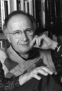
Professor Linus Pauling
Within essentially all undergraduate chemistry classes there appear a multitude of theoretical concepts and equations that render certain constructs quantitative and that connect the laboratory's data to quantities that characterize the structure or other characteristics of the underlying molecules. Where did these concepts and equations come from? Who invented them and how did he or she do so?
Often the experimental chemists who gathered the data on specific chemical reactions or phenomena thought up the concepts or wrote down the equations. In such instances, these chemists may or may not have been practicing theoretical chemistry. If they arrived at an equation by fitting experimental data (e.g., reaction rate constant at various temperatures T) to several functional forms and by trial and error finding which form yielded the best straight line fit (e.g., ln k vs T-1 would likely do so in this example), they might be discovering something useful, but they would not be developing new theory. Only by attempting to explain, in terms of the nature and properties of the constituent atoms and molecules, why this optimal fit applies, would new theory be created. For example, by using more fundamental underlying concepts (e.g., the assumption that a molecule's electrons and nuclei obey the Schrödinger equation or that the nuclei move classically on a potential energy surface that has a pass connecting reactants to products) to derive or suggest why ln k should vary as T-1 would these scientists be practicing the science of theoretical chemistry.
Most of the equations encountered in chemistry text books have been shown to be related to an underlying theoretical picture of atomic and molecular behavior. Hence, most of these equations represent real theory and the people whose names are attached to them practiced theoretical chemistry. However, in modern times, there is far more to this exciting and relatively young area of chemistry than deriving new equations, although doing so remains a mainstay of this discipline. In the subsection entitled Present Day Theoretical Chemistry, we will encounter three distinct avenues along which theory is contributing to the development of chemical science. Most practicing theoretical chemists make contributions along all three avenues, although it is common for most to specialize in one of the three. Moreover, it is not only full-time theoretical chemists who contribute to the advancement of these areas; many chemists whose primary emphasis lies in laboratory research continue to make seminal contributions.
Another development of recent years is the appearance of scientists who specialize in theory to the exclusion of experimental work. In the times of Arrhenius, and later of Linus Pauling and Henry Eyring, most new theoretical developments in chemistry were made by the experimentalists who gathered the laboratory data, although there were some exceptions (e.g., J. Willard Gibbs).
Professor Linus Pauling
During the 1950's and continuing to this day, specialization within all subdisciplines of chemical science has proceeded to an extent that more and more theory is carried out in the hands of professional theoretical chemists who do not have active laboratory research programs. There continue to be practicing experimental chemists (e.g., Dudley Herschbach, Dick Zare, Josef Michl, Michael Morse, and numerous others) who also make major contributions to the theoretical framework of chemistry, and many if not most experimentalists create new theories or models as they interpret their laboratory data.
Professor Dudley Herschbach

Professor Dick Zare (right) at the South Pole

Professor Michael Morse
However, much of today's theoretical research is carried out by
specialists who do not have experimental laboratories but who use
paper, pencil, and computers to do their work. This attribute has
made hiring theoretical chemistry faculty especially attractive to
smaller colleges and universities who can not afford to equip as many
expensive research laboratories, which, in turn, has contributed to
the healthy growth of this field. Let us now consider in more detail
how theory fits into the research and education paradigms of
chemistry.
The rate of a chemical reaction
a A + b B Æ c C + d D
measured at several different temperatures can be used to
determine the rate coefficient k(T) at these temperatures assuming
one has already determined the orders in the rate law (na
and nb
in this example)
rate = k [A]na
[B]nb .
As discussed in most undergraduate
introductory and physical chemistry texts, a plot of ln k(T)
vs T-1 can then be used to extract an activation energy
Ea if the dependence of k on T is assumed to obey the
Arrhenius theoretical model
ln (k) = A - Ea/RT.
During the time of Arrhenius, understanding of the meaning of the parameters A and Ea obtained by analyzing rate data in this manner was limited. It was not known how they related to intrinsic properties of the reacting molecules, although the Arrhenius equation proved a powerful tool for predicting reaction rates over a wide range of temperatures once Ea and A had been determined.
Subsequent to Arrhenius' time, Henry Eyring showed, using the tools of quantum mechanics and statistical mechanics, that the rate of passage of the reacting molecules over the lowest pass or col on their potential energy surface would have a temperature dependence given by the Arrhenius equation. Moreover, he gave expressions for Ea as the height of the pass above the energy of the reactant species and for the pre-exponential A factor in terms of the instantaneous geometry and vibrational frequencies of the reacting molecules when they reach this pass, which is now termed the transition state. Eyring thus put the Arrhenius equation on sound theoretical ground by relating the measured rate and temperature fully to molecule-level quantities.
In this case, the experimental data are the rate determined, for
example, as the rate of disappearance of one of the reacting species
and the temperature T. The theory is embodied in the equation: ln (k)
= A - Ea/RT that allows one to fit the measured data to
extract Ea and A which are, in turn, related through
theory to properties of the molecules at the transition state.
Let us consider another example involving the determination of
molecular geometries; for example, bond lengths in linear molecules.
Using microwave spectroscopy,
an experiment can be performed to measure the frequencies
(nk) of radiation absorbed by a
gaseous sample of a molecule that possesses a dipole moment. One then
uses a theoretical equation such as
EJ,M = J(J+1) h2/(8p2I)
which gives the rotational energy levels of a linear molecule in
terms of the rotational quantum numbers J and M as well as the moment
of inertia of the molecule I and Planck's constant h. Using the
absorption selection rule J Æ J+1
that results because one photon of light carries one unit of angular
momentum, one can then relate each of the absorption frequencies to
differences in neighboring (i.e., J Æ
J+1) energy levels
hnk = h2/(8p2I) {(J+1) (J+2) - J (J+1)} = 2 (J+1) h2/(8p2I).
This theoretical expression suggests that each microwave spectrum
should display a series of evenly spaced absorption lines whose
spacing
h(nk+1 - nk ) = 2 h2/(8p2I)
can be used to extract the moment of inertia I of the molecule,
which is then related to the bond lengths in the molecule. For
example, in a diatomic molecule AB, I is given by
I = {mA mB/(mA + mB)} r2,
where mA and mB are the masses of the atoms A and B and r is the bond length between A and B.
In this example, the experimental data are the frequencies
nk of microwave radiation
absorbed by the molecules. The theory is given in the equation
h(nk+1 - nk
) = 2 h2/(8p2I) that
allows one to extract the molecular property of interest, the bond
length r.
In both of the above examples, the precision with which the measurement is made may be very high, but the accuracy with which the molecule- level property is determined may be more limited if the theoretical equation used to connect the experiment to the molecule is lacking.
Not all such equations have yet been derived, and many that appear in undergraduate and graduate textbooks are based on approximations and are still undergoing refinements by present day theoretical chemists.
In present day theoretical chemistry, much effort is devoted to
making more rigorous the equations we use to effect the
laboratory-to-molecule connections. For example, the equation
EJ,M = J(J+1) h2/(8p2I)
used above is only the most rudimentary expression for the rotational
energy levels of a linear molecule. More sophisticated expressions
take into consideration the dependence of the moment of inertia on
the particular vibrational state (v) the molecule occupies; in
different vibrational states, the average bond lengths are different,
so I depends on the quantum number v:
EJ,M = J(J+1) h2/(8p2Iv).
Moreover, since the rotational energies depend on the bond length
r as r-2, the average rotational energy for a particular
vibrational state v is more properly written in terms of the average
over state v of the quantity 1/r2:
EJ,M = J(J+1) h2/[8p2{mA mB/(mA + mB)} <v| 1/r2 |v>].
Because the molecule has a bond length r that is undergoing
vibrational movement, r certainly is not constant over time; so, what
is the bond length really? This question points at the heart
of an important issue that arises whenever theory is used to relate
experimental measurements to molecule-level properties. Let us pursue
this further to clarify. The average interatomic distance <v| r
|v> experienced by the AB diatomic vibrating in its vth
vibrational level is not equal to the value of r at the minimum of
the AB interatomic potential re. Moreover, the average
<v| 1/r2 |v> that enters into the rotational energy
expression is not equal to re-2 nor is it equal
to <v| r |v>-2. So, what is the real meaning of the
AB molecule's bond length? As this illustration shows, the concept
of bond length, when viewed with more and more scrutiny, is not
uniquely clear. Bond lengths extracted from microwave spectroscopy
data really have to do with average values of r-2.
However, bond lengths of, for example, ionic AB molecules determined
by measuring the dipole
moment m of AB and assuming
m can be related to the unit of charge e
and the average separation between the atomic centers
m = e <v| r |v>
probe the average of r, not of r-2. Hence, different
experimental data, when interpreted in terms of even the most up to
date theoretical equations, can produce different numerical values
for bond lengths because there really is no such thing as a uniquely
defined bond length.
Not only is present day theoretical chemistry making improvements
to equations such as the Arrhenius-Eyring equation and the
rigid-rotor energy equation that have existed for many years, but
theory is attempting to derive equations for cases that do not yet
have even approximate solutions. For example, the low-energy
vibrational levels of "rigid" molecules (i.e., species containing
only strong bonds) such as CH4, H2O, and
NF3 can approximately be represented in terms of
harmonic-oscillator energy expressions, one for each of the 3N-6
vibrational modes (N is the number of atoms in the molecule):
E = Si=1, 3N-6hwi (ni+1/2).
However, for either (a) these same rigid molecules at higher total
vibrational energy (e.g., states whose total vibrational energy is
ca. 50% of the dissociation energy of the weakest bond in the
molecule) or (b) for "floppy" molecules with at least one much weaker
bond such as the van der Waals complex Ar®HCl
or the Na3 trimer (where the pseudo-rotation among the
three Na atoms is a "floppy" vibrational mode), there do not yet
exist widely accepted equations that can be used even as starting
points for adequately describing these vibrational energy levels.
Hence, when the rotational spectra (or rotationally resolved
vibrational spectra) of these molecules are measured in the
laboratory, it remains very difficult to extract accurate geometry
information from such spectra, no matter how high the precision of
the experiments. The missing link in this case is the equation
relating the data to the molecule-level geometry information. Perhaps
a student reading this will come to be the scientist who makes the
needed breakthroughs on this problem.
Oxidation numbers are good examples of quantities that we use to systematize chemical behavior. In NaCl, we assign +1 and -1 oxidation numbers to Na and Cl. In H2O, we assign +1 to H and -2 to O; and in H2O2, we use +1 for H and -1 for O. Finally, in Ti(H2O)6+3 we use +3 for Ti , +1 for H and -2 for O.
We do not believe these oxidation numbers represent the actual charges that the atoms in these molecules possess as they exist in mother nature, although we almost believe so in the NaCl case because here the electronegativity difference between Na and Cl is so large that their bond is nearly ionic. However, in H2O the bonds are covalent, although quite polar, so the O atom certainly does not exist as an essentially intact O-2 dianion in this molecule. Also in Ti(H2O)6+3 , Ti can not exist as an intact Ti+3 ion surrounded by six neutral H2O molecules since the energy (12.6 eV) needed to remove an electron from an H2O molecule would be more than offset by the energy gained (28.1 eV) by reducing Ti+3 to Ti+2, plus the Coulomb repulsion energy then arising between the H2O+ and Ti+2 ions.
Nevertheless, oxidation numbers provide a useful concept which chemists can use both to predict stoichiometries and to suggest the relative electron "richness" of various atomic sites in molecules. The concept of electronegativity, likewise, is one that chemists use to describe the local electron richness of an atomic center in a chemical bond. In the definition suggested by Prof. Robert Mulliken, the University of Chicago molecular spectroscopist and theorist who coined the term "molecular orbital", the electronegativity c of an atom A is related to that atom's ionization potential IP and its electron affinity EA:
cA = 1/2 (IPA + EAA ),
which is often interpreted as saying that an atom's ability to
attract (EA) and to hold (IP) electron density should be so
related.
The relative ability of a molecule to accept (Lewis
acid) or donate (Lewis base) an electron pair is a concept that we
use often to rationalize bond strengths. For example, we suggest that
CO binds to the Fe center in hemoglobin through its Carbon atom end
because (1) the s lone pair on C is less
tightly held than that on O, and (2) the antibonding p*
orbital is more highly localized on C than O as a result of which CO
is both a better s Lewis base using its C
atom end and a better p-acceptor also
using its C atom end.
These rules (R. B. Woodward was one of the U.S.'s most successful and renowned organic chemists; Roald Hoffmann is a theoretical chemist. Hoffmann shared the 1981 Nobel Prize with Kenichi Fukui) allow us to follow the symmetry of the occupied molecular orbitals along a suggested reaction path connecting reactants to products and to then suggest whether a symmetry-imposed additional energy barrier (i.e., above any thermodynamic energy requirement) would be expected. For example, let us consider the disrotatory closing of 1,3-butadiene to produce cyclobutene. The four p orbitals of butadiene, denoted p1 through p4 in the figure shown below, evolve into the s and s* and p and p* orbitals of cyclobutene as the closure reaction proceeds. Along the disrotatory reaction path, a plane of symmetry is preserved (i.e., remains a valid symmetry operation) so it can be used to label the symmetries of the four reactant and four product orbitals. Labeling them as odd (o) or even (e) under this plane and then connecting the reactant orbitals to the product orbitals according to their symmetries, produces the orbital correlation diagram shown below.
Professor Roald Hoffmann
The four p electrons of 1,3-butadiene
occupy the p1 and p2
orbitals in the ground electronic state of this molecule. Because
these two orbitals do not correlate directly to the two orbitals that
are occupied (s and p)
in the ground state of cyclobutene, the Woodward-Hoffmann rules
suggest that this reaction, along a disrotatory path, will encounter
a symmetry-imposed energy barrier. In constrast, the excited
electronic state in which one electron is promoted from p2
to p3 (as, for example, in a
photochemical excitation experiment) does correlate directly to the
lowest energy excited state of the cyclobutene product molecule,
which has one electron in its p orbital
and one in its p* orbital. Therefore,
these same rules suggest that photo-exciting butadiene in the
particular way in which the excitation prootes one electron from
p2 to p3
will produce a chemical reaction to generate cyclobutene.p2
to p3
The advent of computers that can carry out numerical calculations at high speed has opened up new possibilities for theoretical chemistry analogous to what it has done for the automobile, machine, and aerospace industries. For example, the design of new aircraft and rockets used to require much trial and error building and testing. Although the fundamental equations governing thrust, airfoil dynamics, and the like were known, prior to the existence of high speed computers, they could not be numerically solved fast enough to allow engineers to predict the behavior of new aircraft. Today, numerical simulation has replaced much of the trial and error work in these industries. A similar breakthrough has occurred in theoretical chemistry because computers are now powerful enough to permit efficient numerical solution of the underlying equations.
Although the fundamental laws governing the movement of electrons and atomic nuclei in molecules may have been known for many years, the solution of these equations to permit monitoring these motions only became practical due to advances in computer power starting in the 1950s and continuing to this day. For example, early theoretical chemists such as Joe Hirschfelder and Eyring had to use slide rules and tabulated values of special functions to compute the potential energy surface and the classical-mechanics trajectory for the H + H2 Æ H2 + H reaction (which they further approximated by assuming collinear collision geometries). They were able to carry out numerical simulations of this simple reaction, but it required many months of Hirschfelder's Ph. D. education effort. Today, such simulations would require only seconds on a desktop workstation. Moreover, today's higher speed computers permit us to examine much more complicated molecules and reactions via simulation.
Simulation thus involves numerically solving, on a computer using
various tools of numerical analysis, a set of assumed equations
(e.g., as in the Hirschfelder-Eyring case, it may be Newtonian
equations of motion governing the movement of atoms within a molecule
or it may be the Schrödinger equation describing the motions of
electrons within a molecule). The details of such a calculation can
be monitored throughout the calculation to "watch" the molecules as
they undergo their motions. For example, a Newtonian simulation of
the time evolution of a cyclohexane molecule surrounded by methane
solvent molecules can be used to monitor how often the chair confomer
of cyclohexane interconverts into the boat confomer. By probing the
solution to the Newton equation of motion at each time step in the
numerical process, one can extract data such as the chair-to-boat
interconversion rate constant. Let us consider a few more examples of
simulations to further illustrate these points.
In the figures shown below are depicted the average of the square
of the distance R2 that a CH4 molecule has
moved from its original position (R=0) in a length of time t at 250 K
and at 400 K. In the simulations that
produced this numerical data, which were carried out by the
research group of Dick
Boyd my Materials Science and Engineering colleague at Utah,
the CH4 molecule was surrounded by cis- polybutadiene
(cis-PBD) molecules. The average mentioned above involves averaging
over many trajectories with various initial conditions (e.g.,
velocities of the CH4 and PBD selected from
Maxwell-Boltzmann distributions appropriate to 250 K or 400 K). The
equations that were solved to monitor the position of the
CH4 molecule in this example are classical Newtonian
equations of motion. In these equations, several kinds of forces
appear (through gradients of the potential energy F =
- ![]() V):
V):
a. harmonic restoring forces that constrain the bond lengths and internal angles of the CH4 molecule to near their equilibrium positions; because the temperature T is not extremely high, these coordinates are not likely to wander far from their equilibrium values, so this harmonic treatment is probably adequate.
b. attractive van der Waals r-6 and repulsive r-12 potentials between each of the atoms in the CH4 molecule and each of the atoms in each of the PBD molecules.
c. attractive van der Waals and repulsive potentials between each of the atoms in one PBD molecule and those in another PBD molecule.
The specific values of the so-called C6 and C12 parameters that enter into each set of attractive and repulsive potentials:
V = C12/r12 - C6/r6
had been determined from other independent measurements that probed these intermolecular interactions or by quantum chemical calculations of these interaction energies. Implicit in all of these potentials is the assumption that the CH4 and all PBD units are in their ground electronic states. If any of these species were in an excited state, the intermolecular potentials, and hence the forces, involving those species would be different and parameters appropriate to these excited species would have to be used in solving the equations.
When solving the Newton equations on a computer, one uses initial values of the coordinates and momenta of each particle to propagate these coordinates and momenta to later times. This propagation, in its simplest version, calculates the cartesian coordinate qi at the next time in terms of the coordinate at the present time qi0 and the corresponding momentum pi 0
qi (t+dt) = qi 0 + pi 0 /mi dt.
The momenta, are computed as:
pi (t+dt) = pi0 + [V/
The sequence of qi and pi values obtained by iterating on the above equations is called a "trajectory" because it details, in discrete form, the path in coordinate and momentum space that the molecular system follows in time.
These molecular dynamics simulations often consume a great deal of computer time primarily for three reasons:
1. To treat motions that occur on vibrational timescales (e.g.,10-14 sec) for long enough times to monitor diffusion (e.g., 1000 ps) requires using many (e.g., 105 ) time steps in the Newton equations' numerical integration.
2. To evaluate the forces and intermolecular potentials among N atoms requires computer time that scales as N2 (or worse) because these potentials and forces depend on the coordinates of pairs of atoms.
3. To achieve an accurate representation of a realistic experimental system, many trajectories, with initial coordinates and momenta chosen from the appropriate statistical distribution (e.g., the Maxwell-Boltzmann velocity distribution), must be propagated.
For these reasons, it is not difficult to imagine why the CH4
in PBD simulations whose data is shown below are so computer
time intensive.
Mean-squared displacement vs. time for methane diffusing in
cis-PBD at 250 K. The inset is a blow-up of the early time region
showing the 'cage' effect before true diffusion sets in. The
deviations at long time represent increased statistical
noise.
Mean-squared displacement vs. time for methane diffusing in
cis-PBD at 400 K. The inset is a blow-up of the early time
region.
What is learned from the simulation data presented in the above
figures? We note that, although the values of R2 vary in a
"jerky" manner on very short time scales (e.g., 5-50 ps), the general
trend is for R2 to vary linearly with t for longer times
(e.g., > 100 ps). Just as in a laboratory experiment, the data so
generated can be used to extract molecule-level parameters only if
one has available an equation that relates the data to the molecule.
Long ago, Einstein, and
others examined the random (so-called Brownian) motions that
characterize the center-of-mass movement of a molecule embedded in
other molecules at some temperature T. They showed that, for long
times, the mean square distance R2 covered by such a probe
molecule should obey an equation that is linear in time t:
R2 = 2Dt.
Here, D is the diffusion coefficient that characterizes the
molecule as well as the medium through which it diffuses
D = kT/(6pah),
h is the viscosity of the surrounding
molecules (cis-PBD above) and a is the radius of the particle
(CH4) diffusing through the other molecules. So, by
measuring the slopes of the average of R2 vs time plots
shown above, one can extract D at the two temperatures. If
h of cis-PBD is known, one can then
determine the "size" of the diffusing molecules as contained in the
radius value a, which is the molecule-level parameter in this
example.
In addition to classical and quantum dynamical simulations of the time evolution of molecules, theory uses the so-called Monte-Carlo method to simulate the behavior of molecular systems that exist in thermal equilibrium. This theory was developed to provide an efficient evaluation of thermal equilibrium characteristics.
Briefly, the framework of statistical mechanics tells us that the
equilibrium average <A> of any property A that can be expressed
in terms of the coordinates {qi} and momenta
{pi}: A({qi}, {pi}) is equal to the
following ratio of multidimensional integrals
<A> =
Ú A({qi},{pi})exp[-bH({qi},{pi})]dq1...dqNdp1...dpN-----------------------------------------------------------------------------------------
Ú exp[-bH({qi},{pi})]dq1...dqNdp1...dpN
- P({qi}, {pi}) =
- exp[-bH({qi},{pi})]dq1...dqNdp1...dpN
- ---------------------------------------------------------------------
- Ú exp[-bH({qi},{pi})]dq1...dqNdp1...dpN
represents the Boltzmann probability density that the system
realize the particular {qi}, {pi} values. As
such, P is normalized to unity
1 = Ú P({qi},{pi})dq1dqNdp1dpN
and is a positive definite quantity. Because it has these
properties, it was possible for Metropolis and Teller to show that
the above 2N dimensional phase-space integral (N being the number of
geometrical degrees of freedom needed to describe the molecular
system) could be evaluated by executing the following so-called
Metropolis Monte-Carlo
process:
a. Starting with the molecular system having particular values ({qi}, {pi})0 , one randomly selects one of the 2N variables {qi}, {pi}; let us call this variable x for what follows.
b. One alters the selected x by a small amount x Æ x+dx.
c. One computes the change dH in H({qi}, {pi}) that accompanies the change dx in x.
d. One evaluates exp[-b dH] Ü S, which is how the temperature T enters into the simulation.
e. If S > 1 (which means that dH is negative or, in turn, that the potential energy change in dH caused by the small change dx in x is in the "downhill" direction), then one "accepts" the move from x to x + dx, and one then begins this iterative procedure again back at step a.
f. If, on the other hand, S < 1 (which means that dH
is positive), one compares S to a random number R lying between 0.0
and 1.0. If S>R, one accepts the move to x + dx;
if S<R, one rejects the move to x + dx.
In either case, one returns to step a and continues.
This procedure is designed to generate a series of accepted values for the variables {qi}, {pi} that are representative of the normalized Boltzmann probability density P({qi}, {pi}) described above in a manner that is much more efficient than simply dividing each of the 2N variable ranges into, for example, p discrete "chunks" and performing the averaging integral <A> numerically by summing over p chunks in each of 2N dimensions. The latter process would require computer time that scales as p2N . In contrast, the Metropolis process requires time that scales linearly with N (or to a low power of N, Ns , if the evaluation of H, which involves computing the change in the potential energy of interaction of the one particle being moved with all other particles, scales as Ns ). The key efficiency inherent in the Metropolis process lies in how it selects moves to accept. The set of accepted values of ({qi}, {pi}) is weighted heavily exactly where exp (-b H) is large, and weighted lightly where exp (-b H) is small, and the density of points points ({qi}, {pi}) in this space is proportional to exp (-b H).
The Monte-Carlo method is thus a very powerful tool for simulating
molecules that are in equilibrium conditions. In the figures shown
below are the results of such a simulation carried out on NO2
- (H2 O)n clusters
within the author's research group. At each accepted step of
the Monte-Carlo procedure, various information was collected. For
example, the distance from the N atom of the anion to each of the O
atoms of the surrounding water molecules, as well as the angle
between the vector connecting the N atom to a water molecule's O atom
and the C2 symmetry axis of the NO2 -
ion. Collecting such information for a large number of accepted
moves allows one to subsequently make histogram plots that display
how frequently, among the accepted steps, a particular N-to-O
distance R or angle q (defined with 180
deg corresponding to the direction from the N atom to the midpoint
between the two O atoms of the anion) is found. In this manner, one
can simulate the radial and angular distributions of the H2
O molecules that surround an NO2 - ion in
equilibrium at temperature T as shown in the figures below.
The histograms shown above suggest that, for NO2 -
(H2 O)6 , most of the H2 O
molecules reside (most of the time) ca. 5.5 bohr (bohr is a unit of
distance equal to 0.529 Å, the radius of the Hydrogen atom's 1s
orbital) from the N atom, but some reside further out. They also show
that all six of the solvent molecules tend to reside at angles
greater than ca. 50 deg. A conclusion that has been drawn from these
data is that a second hydration layer (e.g., the solvent molecules
residing beyond 6 bohr) begins to form before the first layer is
completed (because solvent molecules are not found at angles between
0 deg and ca. 50 deg.
The chief drawback of the Metropolis Monte-Carlo method lies in the statistical errors which limit its accuracy. The percent error in any computed equilibrium average varies as the inverse of square root of the number M of accepted Monte-Carlo moves (n.b., in the two figures shown above, ca. 1,000,000 moves were carried out). Hence, if 100,000 moves are used to achieve a radial distribution function whose statistical accuracy is lacking, one would have to carry out a simulation with 10,000,000 moves to cut the error down by a factor of 10; that is, it would require 100 times the effort to reduce the error a factor of 10.
In closing this section on simulations, it is important to stress that theory does not replace real laboratory measurements via its computer simulations, just as flight simulators or aircraft design simulations do not replace the need for pilot training or aircraft testing. The equations and underlying models that are used in any simulation never replicate nature's real behavior (although we strive to develop models that are more and more accurate pictures of nature). So, the data that is obtained in a computer experiment is always inaccurate because of imperfections in the theoretical model. The computer experiment's strengths are:
1. That one can monitor the molecule's time evolution in much greater detail than in a real lab experiment (i.e., one can "watch" each and every aspect of the molecules' movements if one is carrying out classical simulations or, analogously, one can monitor individual quantum state populations as time progresses in quantal simulations);
2. That one can gain a measure of theory's accuracy (and thus the need to effect improvements in the underlying theory) by comparing predictions of computer simulations with real lab data.
Having made it clear that theoretical simulation can not fully
replace experimental measurement, I think it also important to stress
that theory can often be carried out on species that (a) may be very
difficult to prepare and isolate in the laboratory (e.g., reactive
radicals and unstable molecules) or (b) have not yet been observed in
nature. The latter area, that of using theory to predict and examine
the chemical and physical behavior of molecules, ions, and materials
that have yet to be synthesized or observed, is one of the most
exciting characteristics of theoretical chemistry. To me, this allows
theoretical simulation to be used to suggest new species to the
experimental chemist for possible simulation, thus making us part of
thep process of creating new molecules and materials.